May 15, 2020
Bug Bois (Project 1): Sloan Dickson (JSD2385)
Introduciton
These datasets are from the iNaturalist website which collects wildlife data. The website collects this data from members who identify wildlife in their daily lives and submit the location, species identification, specimen descriptions, and photographs/audio recordings as well as a number of other variables. The iNaturalist community then looks at these submissions and tries to correctly identify the species and give more detail on its taxonomy and whether it belongs in that location or is invasive. The datasets I drew from this website are recordings of beetle sightings from the world (without USA data) in the first 6 months of 2019 (if I collected anymore data I would not have been able to export it due to size) and all insect sightings in the USA from all of 2019. They contain 38 and 37 variables respectfully, which are listed below using the names function (ID, time observed, quality_grade, etc.) The variables this project focuses on are the taxonomic variables, the time zone (which I will use, the accuracy of the and the number of agreements and disagreements observed. This dataset drew my attention because I have always liked to learn about entomology and this dataset both provides interesting observations of insects from around the world and shows what places in the world are most interested in entomology. I will be joining these datasets to only see beetle observations (USA and worldwide) and will be assessing the data for the following questions: - Which families or species have the most discussion/disagreements on identification overall? - Does taxon predict discussion? - Are there differences in the amount of discussion in different parts of the world (North America and Central America vs other parts of the world)? - Are there different amounts of agreements/disagreements depending on the accuracy of the location data (higher values for positional accuracy are less accurate as it measures)? Are people more or less likely to consider species guesses valid depending on this variable?
(A side note: After beginning working with this dataset, I realized that a large number of my numeric variables were essentially useless without individually editing their observations to make them useful. For example, the location information was all clumped together at the discretion of the person inputting the observation. This means that each observation was formatted differently (some added city, state, and even the street they were on while others just listed their country). This format makes it almost impossible to use as a grouping method, so I had to adapt the time_zone variable to give an estimate for location. Because a number of the numeric variables were formatted so irregularly, I had to resort to numeric variables I previously never considered such as positional_accuracy.)
Let’s load in the datasets.
library(tidyverse)
library(ggplot2)
library(GGally)
library(kableExtra)
library(plotly)
library(cluster)

world_beetles <- read.csv("beetles_2019.csv")
usa_insects <- read.csv("usa_insects.csv")

#These datasets are both quite large in number of observations and in the number of variables and will likely need to be edited to be more manageable.
This dataset contains 8462 observations from 2019/01/01 to 2019/06/31
glimpse(world_beetles)## Observations: 8,462
## Variables: 38
## $ id <int> 18177129, 19251162, 19342293, 193432…
## $ observed_on_string <fct> 2019-03-29, 2019-01-03 4:54:22 p.m. …
## $ observed_on <fct> 2019-03-29, 2019-01-03, 2019-01-01, …
## $ time_observed_at <fct> , 2019-01-03 16:54:22 UTC, 2018-12-3…
## $ time_zone <fct> Quito, Edinburgh, Brisbane, Asia/Mag…
## $ out_of_range <fct> , , , , , , , , , , , , , , , , , , …
## $ user_login <fct> fcheca, bee-man, pierswarmers, lileb…
## $ created_at <fct> 2018-11-06 20:20:53 UTC, 2018-12-27 …
## $ updated_at <fct> 2019-03-30 20:01:38 UTC, 2019-01-03 …
## $ quality_grade <fct> research, needs_id, research, resear…
## $ description <fct> , , Huge beetle. About 10cm long. Ve…
## $ id_please <fct> false, false, false, false, false, f…
## $ num_identification_agreements <int> 3, 0, 2, 1, 1, 1, 3, 1, 1, 3, 2, 4, …
## $ num_identification_disagreements <int> 0, 0, 0, 0, 0, 0, 0, 0, 0, 0, 0, 1, …
## $ captive_cultivated <fct> false, false, false, false, false, f…
## $ oauth_application_id <int> NA, 2, 3, 3, 2, 111, 3, NA, 3, 111, …
## $ place_guess <fct> "Guajalito", "56A Danecourt Rd, Pool…
## $ latitude <dbl> -0.3305124, 50.7265199, -26.4110500,…
## $ longitude <dbl> -78.609349, -1.958835, 152.829942, N…
## $ positional_accuracy <int> 244, 44, 165, 10988, 4, NA, 6, 15, 0…
## $ geoprivacy <fct> , , , private, , obscured, , , , obs…
## $ taxon_geoprivacy <fct> , , , , , , , , , , , , , , , , , , …
## $ coordinates_obscured <fct> false, false, false, true, false, tr…
## $ positioning_method <fct> , gps, , , , , , , , , , , , , , , ,…
## $ positioning_device <fct> , gps, , , , , , , , , , , , , , , ,…
## $ species_guess <fct> Hippodamia convergens, Cockchafer Be…
## $ scientific_name <fct> Hippodamia convergens, Melolontha, A…
## $ common_name <fct> Convergent Lady Beetle, Cockchafer B…
## $ iconic_taxon_name <fct> Insecta, Insecta, Insecta, Insecta, …
## $ taxon_id <int> 48987, 48199, 201855, 341892, 371066…
## $ taxon_kingdom_name <fct> Animalia, Animalia, Animalia, Animal…
## $ taxon_phylum_name <fct> Arthropoda, Arthropoda, Arthropoda, …
## $ taxon_class_name <fct> Insecta, Insecta, Insecta, Insecta, …
## $ taxon_order_name <fct> Coleoptera, Coleoptera, Coleoptera, …
## $ taxon_family_name <fct> Coccinellidae, Scarabaeidae, Ceramby…
## $ taxon_genus_name <fct> Hippodamia, Melolontha, Agrianome, C…
## $ taxon_species_name <fct> Hippodamia convergens, , Agrianome s…
## $ taxon_subspecies_name <fct> , , , , , , , , , , , , , , , , , , …There are 38 variables as seen below
names(world_beetles)## [1] "id" "observed_on_string"
## [3] "observed_on" "time_observed_at"
## [5] "time_zone" "out_of_range"
## [7] "user_login" "created_at"
## [9] "updated_at" "quality_grade"
## [11] "description" "id_please"
## [13] "num_identification_agreements" "num_identification_disagreements"
## [15] "captive_cultivated" "oauth_application_id"
## [17] "place_guess" "latitude"
## [19] "longitude" "positional_accuracy"
## [21] "geoprivacy" "taxon_geoprivacy"
## [23] "coordinates_obscured" "positioning_method"
## [25] "positioning_device" "species_guess"
## [27] "scientific_name" "common_name"
## [29] "iconic_taxon_name" "taxon_id"
## [31] "taxon_kingdom_name" "taxon_phylum_name"
## [33] "taxon_class_name" "taxon_order_name"
## [35] "taxon_family_name" "taxon_genus_name"
## [37] "taxon_species_name" "taxon_subspecies_name"This dataset contains 8462 observations from 2019/01/01 to 2019/12/31
glimpse(usa_insects)## Observations: 32,920
## Variables: 37
## $ id <int> 5942947, 19354339, 19360615, 1936103…
## $ observed_on_string <fct> Wed Apr 17 2019 15:26:11 GMT-0600 (M…
## $ observed_on <fct> 2019-04-17, 2019-01-01, 2019-01-01, …
## $ time_observed_at <fct> 2019-04-17 21:26:11 UTC, 2019-01-01 …
## $ time_zone <fct> Mountain Time (US & Canada), Eastern…
## $ out_of_range <fct> , , , , , , , , , , , , , , , , , , …
## $ created_at <fct> 2017-04-24 21:58:54 UTC, 2019-01-01 …
## $ updated_at <fct> 2019-04-18 18:56:43 UTC, 2019-06-26 …
## $ quality_grade <fct> needs_id, needs_id, needs_id, needs_…
## $ description <fct> "Shiny green insect (fly). Has black…
## $ id_please <fct> false, false, false, false, false, f…
## $ num_identification_agreements <int> 2, 0, 0, 0, 3, 2, 1, 0, 1, 0, 0, 0, …
## $ num_identification_disagreements <int> 0, 0, 0, 0, 0, 0, 0, 0, 0, 0, 0, 0, …
## $ captive_cultivated <fct> false, false, false, false, false, f…
## $ oauth_application_id <int> 3, 3, 2, 3, 2, 3, 2, 3, NA, 2, 3, 2,…
## $ place_guess <fct> "University of Texas at El Paso, El …
## $ latitude <dbl> 31.77062, 43.67979, 41.07834, 30.143…
## $ longitude <dbl> -106.50356, -72.31209, -73.78816, -8…
## $ positional_accuracy <int> 65, 50, 1393, 10, NA, 26, 9, 20, 187…
## $ geoprivacy <fct> , , , , , , , , obscured, , , , , , …
## $ taxon_geoprivacy <fct> , , , , , , , , , , , , , , , , , , …
## $ coordinates_obscured <fct> false, false, false, false, false, f…
## $ positioning_method <fct> , , , , gps, , , , , gps, , gps, , ,…
## $ positioning_device <fct> , , , , gps, , , , , gps, , gps, , ,…
## $ species_guess <fct> "Blow Flies", "", "moth", "", "Coleo…
## $ scientific_name <fct> Calliphoridae, Insecta, Insecta, Ins…
## $ common_name <fct> Blow Flies, Insects, Insects, Insect…
## $ iconic_taxon_name <fct> Insecta, Insecta, Insecta, Insecta, …
## $ taxon_id <int> 61860, 47158, 47158, 47158, 174234, …
## $ taxon_kingdom_name <fct> Animalia, Animalia, Animalia, Animal…
## $ taxon_phylum_name <fct> Arthropoda, Arthropoda, Arthropoda, …
## $ taxon_class_name <fct> Insecta, Insecta, Insecta, Insecta, …
## $ taxon_order_name <fct> Diptera, , , , Lepidoptera, Hymenopt…
## $ taxon_family_name <fct> Calliphoridae, , , , Gelechiidae, Fo…
## $ taxon_genus_name <fct> , , , , Coleotechnites, , Carausius,…
## $ taxon_species_name <fct> , , , , , , Carausius morosus, , Dan…
## $ taxon_subspecies_name <fct> , , , , , , , , , , , , , , , , , , …There are 37 Variables as seen below.
names(usa_insects)## [1] "id" "observed_on_string"
## [3] "observed_on" "time_observed_at"
## [5] "time_zone" "out_of_range"
## [7] "created_at" "updated_at"
## [9] "quality_grade" "description"
## [11] "id_please" "num_identification_agreements"
## [13] "num_identification_disagreements" "captive_cultivated"
## [15] "oauth_application_id" "place_guess"
## [17] "latitude" "longitude"
## [19] "positional_accuracy" "geoprivacy"
## [21] "taxon_geoprivacy" "coordinates_obscured"
## [23] "positioning_method" "positioning_device"
## [25] "species_guess" "scientific_name"
## [27] "common_name" "iconic_taxon_name"
## [29] "taxon_id" "taxon_kingdom_name"
## [31] "taxon_phylum_name" "taxon_class_name"
## [33] "taxon_order_name" "taxon_family_name"
## [35] "taxon_genus_name" "taxon_species_name"
## [37] "taxon_subspecies_name"Tidying the Datasets
To tidy this dataset, I will remove unnecessary variables who will just clutter the data (such as “username” and “observed_on_string”) these pieces of data are not the interest or are not useful. I am not going to use the time or date variables as the way they are input by users is inconsistent (ie: day, month year vs moth day year). I also will remove all the rows with NAs . Next I will create a coordinates variable which combines latitude and longitude while separating the variable "taxon_species _name" into “Genus” and “Species” so I can work with these variables more easily. As my datasets are already neat in the sense that they have one row per observation, I will not be able to use pivot longer or pivot wider in the raw data.
To tidy I will be removing non-essential variables from each dataset
beetles2 <- world_beetles %>% select(id, time_zone, observed_on, description,quality_grade, num_identification_agreements, num_identification_disagreements, captive_cultivated, place_guess, latitude, longitude, positional_accuracy, species_guess, scientific_name, common_name, taxon_order_name, taxon_family_name, taxon_species_name)
usa2 <- usa_insects %>% select(id, time_zone, observed_on, description,quality_grade, num_identification_agreements, num_identification_disagreements, captive_cultivated, place_guess, latitude, longitude, positional_accuracy, species_guess, scientific_name, common_name, taxon_order_name, taxon_family_name, taxon_species_name)
I am going to remove all rows with NAs from each datset to make them easier to work with
beetles3 <- beetles2 %>% filter(complete.cases(beetles2))
usa3 <- usa2 %>% filter(complete.cases(usa2))

(beetles2 %>% count())-(beetles3 %>% count())
## n
## 1 2257#2257 observations were lost when nas were removed from the beetles dataset
(usa2 %>% count())-(usa3 %>% count())## n
## 1 10852#10852 observations were lost when nas were removed from the beetles datasetNext I will combine the longitude and latitude columns and separate the genus and species into 2 columns
beetles4 <- beetles3 %>%
  unite(latitude, longitude, col="coordinates",sep=",") %>%
  separate("taxon_species_name",into=c("Genus","Species"))
usa4 <- usa3 %>%
  unite(latitude, longitude, col="coordinates",sep=",") %>%
  separate("taxon_species_name",into=c("Genus","Species"))
The data is now tidy enough to join
glimpse(beetles4)## Observations: 6,205
## Variables: 18
## $ id <int> 18177129, 19251162, 19342293, 193436…
## $ time_zone <fct> Quito, Edinburgh, Brisbane, Nuku'alo…
## $ observed_on <fct> 2019-03-29, 2019-01-03, 2019-01-01, …
## $ description <fct> , , Huge beetle. About 10cm long. Ve…
## $ quality_grade <fct> research, needs_id, research, needs_…
## $ num_identification_agreements <int> 3, 0, 2, 1, 3, 1, 1, 4, 1, 2, 1, 1, …
## $ num_identification_disagreements <int> 0, 0, 0, 0, 0, 0, 0, 1, 0, 0, 0, 0, …
## $ captive_cultivated <fct> false, false, false, false, false, f…
## $ place_guess <fct> "Guajalito", "56A Danecourt Rd, Pool…
## $ coordinates <chr> "-0.3305123546,-78.6093493434", "50.…
## $ positional_accuracy <int> 244, 44, 165, 4, 6, 15, 0, 10, 45045…
## $ species_guess <fct> Hippodamia convergens, Cockchafer Be…
## $ scientific_name <fct> Hippodamia convergens, Melolontha, A…
## $ common_name <fct> Convergent Lady Beetle, Cockchafer B…
## $ taxon_order_name <fct> Coleoptera, Coleoptera, Coleoptera, …
## $ taxon_family_name <fct> Coccinellidae, Scarabaeidae, Ceramby…
## $ Genus <chr> "Hippodamia", "", "Agrianome", "", "…
## $ Species <chr> "convergens", NA, "spinicollis", NA,…glimpse(usa4)## Observations: 22,068
## Variables: 18
## $ id <int> 5942947, 19354339, 19360615, 1936103…
## $ time_zone <fct> Mountain Time (US & Canada), Eastern…
## $ observed_on <fct> 2019-04-17, 2019-01-01, 2019-01-01, …
## $ description <fct> "Shiny green insect (fly). Has black…
## $ quality_grade <fct> needs_id, needs_id, needs_id, needs_…
## $ num_identification_agreements <int> 2, 0, 0, 0, 2, 1, 0, 1, 0, 0, 0, 0, …
## $ num_identification_disagreements <int> 0, 0, 0, 0, 0, 0, 0, 0, 0, 0, 0, 0, …
## $ captive_cultivated <fct> false, false, false, false, false, f…
## $ place_guess <fct> "University of Texas at El Paso, El …
## $ coordinates <chr> "31.7706246942,-106.5035607347", "43…
## $ positional_accuracy <int> 65, 50, 1393, 10, 26, 9, 20, 187, 33…
## $ species_guess <fct> "Blow Flies", "", "moth", "", "Myrmi…
## $ scientific_name <fct> Calliphoridae, Insecta, Insecta, Ins…
## $ common_name <fct> Blow Flies, Insects, Insects, Insect…
## $ taxon_order_name <fct> Diptera, , , , Hymenoptera, Phasmida…
## $ taxon_family_name <fct> Calliphoridae, , , , Formicidae, Lon…
## $ Genus <chr> "", "", "", "", "", "Carausius", "",…
## $ Species <chr> NA, NA, NA, NA, NA, "morosus", NA, "…Joining the Datasets
To join these datasets, a left join will be conducted with world_beetles as the base. This means the dataset will lose observations from the usa_insects that are not beetles. This does not give us the full picture of the insect observations for the United States, but it does allow the project to focus on only the beetles. The observations lost might include more information about identification disputes and positional accuracy trends for iNaturalist users within the United States, but this allows a closer look into those variables and there association to beetle sightings alone.
How many Observations were in the original datasets?
count(beetles4)+count(usa4)## n
## 1 2827328273 observations total.
###Left join
totalbeetlebois <- beetles4 %>% left_join(usa4)(count(beetles4)+count(usa4))-count(totalbeetlebois)## n
## 1 2206822068 observations were lost in the process.
count(totalbeetlebois)## # A tibble: 1 x 1
## n
## <int>
## 1 62056205 observations remain.
Wrangling
I will first filter out all abservations with no identification comparisons for the insects
names(totalbeetlebois)## [1] "id" "time_zone"
## [3] "observed_on" "description"
## [5] "quality_grade" "num_identification_agreements"
## [7] "num_identification_disagreements" "captive_cultivated"
## [9] "place_guess" "coordinates"
## [11] "positional_accuracy" "species_guess"
## [13] "scientific_name" "common_name"
## [15] "taxon_order_name" "taxon_family_name"
## [17] "Genus" "Species"I want a nonzero number of identifications in both the agreements and disagreements categories
test1<-totalbeetlebois %>% filter(num_identification_agreements > 0)
test2<-totalbeetlebois %>% filter(num_identification_disagreements > 0)
Now I will join both of my tests into a new dataset
idbugs <- test1 %>% full_join(test2)Now the only observations remaining are those who have been graded.
###Now I will create a numeric variable from time zone which categorizes whether the obsevation is the North/Central America or not (0=NA/CA, 1=Not NA/CA)
idbugs <- idbugs %>%
  mutate(timezone=case_when(time_zone %in%
                              c("Eastern Time (US & Canada)","Central Time (US & Canada)", "Hawaii",
                                "Pacific Time (US & Canada)","Mountain Time (US & Canada)", "Arizona",
                                "Alaska", "America/Los_Angeles", "America/New_York") ~ 0,
                            time_zone %in% c("Quito", "Brisbane", "Nuku'alofaAsia/Magadan", "Wellington",
                                             "Australia/Perth", "Mid-Atlantic", "Europe/London","Jerusalem",
                                             "Amsterdam","Africa/Johannesburg", "Chennai", "UTC", "Osaka",
                                             "Paris", "Sydney", "Santiago", "Bangkok", "Samoa", "Baghdad",
                                             "West Central Africa", "Pretoria", "Singapore", "Athens",
                                             "Ekaterinburg", "Hong Kong", "Almaty", "Vienna",
                                             "Central America", "Buenos Aires", "London", "Lima", "Brasilia",
                                             "Jakarta", "Bogota", "Kuala Lumpur","Auckland", "Perth",
                                             "Casablanca", "Adelaide", "Mexico City", "Melbourne", "Rome",
                                             "Kyiv", "Stockholm", "Nairobi", "Taipei", "Berlin", "Madrid",
                                             "Atlantic Time (Canada)", "Beijing", "Prague", "Tijuana",
                                             "Edinburgh", "Montevideo", "Copenhagen", "Lisbon", "Abu Dhabi",
                                             "Bern", "Belgrade", "Monterrey", "Mazatlan", "La Paz", "Brussels",
                                             "Guadalajara", "Istanbul", "Hobart", "Pacific/Majuro", "Moscow",
                                             "Yerevan", "Vilnius", "New Delhi", "Tokyo", "Zagreb", "Sofia",
                                             "Seoul", "Ljubljana", "Sri Jayawardenepura", "Warsaw",
                                             "Bucharest", "Bratislava", "Chihuahua",
                                             "Atlantic/Cape_Verde" ,"Islamabad", "American Samoa",
                                             "Cairo") ~ 1)) %>% na.omit() %>% glimpse()
## Observations: 3,943
## Variables: 19
## $ id <int> 18177129, 19342293, 19345676, 193465…
## $ time_zone <chr> "Quito", "Brisbane", "Wellington", "…
## $ observed_on <chr> "2019-03-29", "2019-01-01", "2019-01…
## $ description <chr> "", "Huge beetle. About 10cm long. V…
## $ quality_grade <fct> research, research, research, resear…
## $ num_identification_agreements <int> 3, 2, 1, 4, 1, 1, 1, 1, 1, 1, 1, 2, …
## $ num_identification_disagreements <int> 0, 0, 0, 1, 0, 0, 0, 0, 0, 0, 0, 0, …
## $ captive_cultivated <fct> false, false, false, false, false, f…
## $ place_guess <chr> "Guajalito", "4568, Federal, QLD, AU…
## $ coordinates <chr> "-0.3305123546,-78.6093493434", "-26…
## $ positional_accuracy <int> 244, 165, 15, 10, 198, 10, 5, 4, 165…
## $ species_guess <chr> "Hippodamia convergens", "Poinciana …
## $ scientific_name <chr> "Hippodamia convergens", "Agrianome …
## $ common_name <chr> "Convergent Lady Beetle", "Poinciana…
## $ taxon_order_name <chr> "Coleoptera", "Coleoptera", "Coleopt…
## $ taxon_family_name <chr> "Coccinellidae", "Cerambycidae", "Oe…
## $ Genus <chr> "Hippodamia", "Agrianome", "Thelypha…
## $ Species <chr> "convergens", "spinicollis", "lineat…
## $ timezone <dbl> 1, 1, 1, 1, 0, 1, 0, 1, 1, 0, 1, 0, …What is the ratio of agreements to disagreements in identification for each observation?
Creating a new variable called “acuracy_ratio”
idbugs <- idbugs %>% mutate(num_identification_agreements1=(num_identification_agreements+1)) %>% mutate(num_identification_disagreements1=(num_identification_disagreements+1))%>% mutate(accuracy_ratio = num_identification_agreements1/num_identification_disagreements1)What is the observation with the highest number of disagreements in identification?
idbugs %>% select(id, Genus, Species, num_identification_disagreements) %>% arrange(desc(num_identification_disagreements))## id Genus Species num_identification_disagreements
## 1 20357446 Thelyphassa lineata 2
## 2 19346580 Aspidimorpha miliaris 1
## 3 19425467 Dienerella costulata 1
## 4 19437752 Cheilomenes propinqua 1
## 5 19471161 Trypoxylus dichotomus 1
## 6 19597528 Harmonia axyridis 1
## 7 19627114 Harmonia dimidiata 1
## 8 19691690 Harmonia axyridis 1
## 9 19829972 Alobates pensylvanicus 1
## 10 20051896 Scolypopa australis 1
## 11 20078171 Carabus granulatus 1
## 12 20164619 Hippodamia convergens 1
## 13 20302656 Copris hispanus 1
## 14 20310486 Harmonia axyridis 1
## 15 20315041 Tanystoma maculicolle 1
## 16 20320009 Peltotrupes profundus 1
## 17 20416205 Hemisphaerota cyanea 1
## 18 20429563 Harmonia axyridis 1
## 19 20489440 Meloe proscarabaeus 1
## 20 20652077 Typhaeus typhoeus 1
## 21 20725176 Oplostomus fuligineus 1
## 22 20735333 Eleodes osculans 1
## 23 20833414 Coptocycla texana 1
## 24 20884876 Coccinella californica 1
## 25 20914239 Cysteodemus armatus 1
## [ reached 'max' / getOption("max.print") -- omitted 3918 rows ]Observation 20357446 - Thelyphassa lineata
Now to make it easier to tidy later, I am adjusting the names.
idbugs <- rename(idbugs, agreements=num_identification_agreements)
idbugs <- rename(idbugs, disagreements=num_identification_disagreements)
idbugs <- rename(idbugs, positionalaccuracy=positional_accuracy)
idbugs <- rename(idbugs, accuracyratio=accuracy_ratio)
How many distinct outcomes are there of each variable?
idbugs %>% summarize_all(n_distinct)## id time_zone observed_on description quality_grade agreements disagreements
## 1 3943 90 90 843 3 9 3
## captive_cultivated place_guess coordinates positionalaccuracy species_guess
## 1 2 2753 3792 608 859
## scientific_name common_name taxon_order_name taxon_family_name Genus Species
## 1 603 475 8 68 430 527
## timezone num_identification_agreements1 num_identification_disagreements1
## 1 2 9 3
## accuracyratio
## 1 11Now I will create summary statistics of each numeric variable
idbugs %>% names()## [1] "id" "time_zone"
## [3] "observed_on" "description"
## [5] "quality_grade" "agreements"
## [7] "disagreements" "captive_cultivated"
## [9] "place_guess" "coordinates"
## [11] "positionalaccuracy" "species_guess"
## [13] "scientific_name" "common_name"
## [15] "taxon_order_name" "taxon_family_name"
## [17] "Genus" "Species"
## [19] "timezone" "num_identification_agreements1"
## [21] "num_identification_disagreements1" "accuracyratio"idbugs %>% select(-id) %>% select(-num_identification_agreements1) %>% select(-num_identification_disagreements1) %>% summarize_if(is.numeric, mean, na.rm=T)## agreements disagreements positionalaccuracy timezone accuracyratio
## 1 1.747654 0.01470961 4469.378 0.471722 2.718996idbugs %>% select(-id) %>% select(-num_identification_agreements1) %>% select(-num_identification_disagreements1) %>% summarize_if(is.numeric, sd, na.rm=T)## agreements disagreements positionalaccuracy timezone accuracyratio
## 1 0.9171565 0.1224919 87717.01 0.499263 0.9057776idbugs %>% select(-id) %>% select(-num_identification_agreements1) %>% select(-num_identification_disagreements1) %>% summarize_if(is.numeric, funs(n = n()))## agreements_n disagreements_n positionalaccuracy_n timezone_n accuracyratio_n
## 1 3943 3943 3943 3943 3943idbugs %>% select(-id) %>% select(-num_identification_agreements1) %>% select(-num_identification_disagreements1) %>% summarize_if(is.numeric, n_distinct)## agreements disagreements positionalaccuracy timezone accuracyratio
## 1 9 3 608 2 11idbugs %>% summarize_if(is.numeric, list(Q3=quantile), probs=.75, na.rm=T)## id_Q3 agreements_Q3 disagreements_Q3 positionalaccuracy_Q3 timezone_Q3
## 1 21628623 2 0 128.5 1
## num_identification_agreements1_Q3 num_identification_disagreements1_Q3
## 1 3 1
## accuracyratio_Q3
## 1 3idbugs %>% summarize_if(is.numeric, list(Q1=quantile), probs=.25, na.rm=T)## id_Q1 agreements_Q1 disagreements_Q1 positionalaccuracy_Q1 timezone_Q1
## 1 20351936 1 0 7 0
## num_identification_agreements1_Q1 num_identification_disagreements1_Q1
## 1 2 1
## accuracyratio_Q1
## 1 2idbugs %>% summarize_all(n_distinct)## id time_zone observed_on description quality_grade agreements disagreements
## 1 3943 90 90 843 3 9 3
## captive_cultivated place_guess coordinates positionalaccuracy species_guess
## 1 2 2753 3792 608 859
## scientific_name common_name taxon_order_name taxon_family_name Genus Species
## 1 603 475 8 68 430 527
## timezone num_identification_agreements1 num_identification_disagreements1
## 1 2 9 3
## accuracyratio
## 1 11Summary of the dataset
After calculating the summary statistics for each variable a few notes can be made. The first is that the average number of agreements in identification is higher than that of the disagreements (1.747654 and 0.01470961 respectfully). In addition, the id agreements has a greater standard deviation of 0.9171565 compared to the disagreements’ 0.1224919. This difference in variance is also reflected in the IQR. The variable positional accuracy has a rather high mean of 4469.378 with a high standard deviation of 87717.01.
Correlation matrix among numeric variables
cor_idbugs <- idbugs %>% select_if(is.numeric) %>% select(-num_identification_agreements1,-num_identification_disagreements1, -id) %>% na.omit %>% cor
library(kableExtra)
cor_idbugs %>% kable() %>%
kable_styling(bootstrap_options = c("striped", "hover", "condensed"))| agreements | disagreements | positionalaccuracy | timezone | accuracyratio | |
|---|---|---|---|---|---|
| agreements | 1.0000000 | 0.1594994 | -0.0184377 | 0.1159875 | 0.9641577 |
| disagreements | 0.1594994 | 1.0000000 | -0.0024875 | 0.0233956 | -0.1022066 |
| positionalaccuracy | -0.0184377 | -0.0024875 | 1.0000000 | 0.0025414 | -0.0180167 |
| timezone | 0.1159875 | 0.0233956 | 0.0025414 | 1.0000000 | 0.1111645 |
| accuracyratio | 0.9641577 | -0.1022066 | -0.0180167 | 0.1111645 | 1.0000000 |
Summary of Correlations
The correlations amongst all of the numeric variables are rather low. The highest correlation between variables is between the id accuracy ratio and the id agreements. This is due to the fact that they are inherently related as the accuracy ratio is made up of the combined agreements and disagreements. The other variables have correlations of lower magnitude than .2 which suggests that there is not a relationship.
Now I will create summary statistics of each variable by the Genus and Species of the beetles.
I want to answer the questions: Are some species more likely to have disagreements in their identification? Are some species more likely to have issues with higher accuracy? *Which Species had the highest number of observations?
Creating Summary stats Individually
genusspecies_means <- idbugs %>%
  group_by(Genus, Species) %>%
  select(-id) %>%
  select(-num_identification_agreements1) %>%
  select(-num_identification_disagreements1) %>%
  summarize_if(is.numeric, mean, na.rm=T) %>%
  mutate_if(is.numeric, round)

genusspecies_sd <- idbugs %>%
  group_by(Genus, Species) %>%
  select(-id) %>%
  select(-num_identification_agreements1) %>%
  select(-num_identification_disagreements1) %>%
  summarize_if(is.numeric, sd, na.rm=T) %>%
  mutate_if(is.numeric, round)

genusspecies.n <- idbugs %>%
  group_by(Genus, Species) %>%
  select(-id) %>%
  select(-num_identification_agreements1) %>%
  select(-num_identification_disagreements1) %>%
  summarize_if(is.numeric, funs(n = n())) %>%
  mutate_if(is.numeric, round)

genusspecies.distinct <- idbugs %>%
  group_by(Genus, Species) %>%
  select(-id) %>%
  select(-num_identification_agreements1) %>%
  select(-num_identification_disagreements1) %>%
  summarize_if(is.numeric, funs(n = n())) %>%
  mutate_if(is.numeric, n_distinct)

genusspecies.Q3 <- idbugs %>%
  group_by(Genus, Species) %>%
  select(-id) %>%
  select(-num_identification_agreements1) %>%
  select(-num_identification_disagreements1) %>%
  summarize_if(is.numeric, list(Q3=quantile), probs=.75, na.rm=T) %>%
  mutate_if(is.numeric, round)

genusspecies.Q1 <- idbugs %>%
  group_by(Genus, Species) %>%
  select(-id) %>%
  select(-num_identification_agreements1) %>%
  select(-num_identification_disagreements1) %>%
  summarize_if(is.numeric, list(Q1=quantile), probs=.25, na.rm=T) %>%
  mutate_if(is.numeric, round)
Combining all of these summary stats
genspec_m_sd <- left_join(genusspecies_means, genusspecies_sd, by=c("Species","Genus"), suffix=c(".mean",".sd"))
genspec_n_dist <- left_join(genusspecies.n, genusspecies.distinct, by=c("Species","Genus"), suffix=c(".n",".distinct"))
genspec_Q1_Q3 <- left_join(genusspecies.Q1, genusspecies.Q3, by=c("Species","Genus"), suffix=c(".Q1",".Q3"))

genusspecies_summary <- genspec_m_sd %>% full_join(genspec_n_dist) %>% full_join(genspec_Q1_Q3)
Removing the N/A rows and columns from genusspecies_summary
genusspecies_summary <- genusspecies_summary %>% arrange(Species)
genusspecies_summary <- genusspecies_summary %>% arrange(Species) %>% slice(4:1800)
genusspecies_summary <- genusspecies_summary %>% na.omit()

genusspecies_summary <- genusspecies_summary %>% na.omit()

glimpse(genusspecies_summary)
## Observations: 31
## Variables: 32
## Groups: Genus [12]
## $ Genus <chr> "Aspidimorpha", "Chilocorus", "Cicindel…
## $ Species <chr> "sanctaecrucis", "stigma", "formosa", "…
## $ agreements.mean <dbl> 2, 1, 2, 2, 3, 4, 1, 2, 2, 2, 2, 2, 2, …
## $ disagreements.mean <dbl> 0, 0, 0, 0, 0, 0, 0, 0, 0, 0, 0, 0, 0, …
## $ positionalaccuracy.mean <dbl> 159, 83, 8, 10, 697, 496, 142, 380, 113…
## $ timezone.mean <dbl> 0, 0, 0, 0, 0, 0, 0, 0, 0, 0, 0, 0, 0, …
## $ accuracyratio.mean <dbl> 2, 2, 2, 3, 4, 4, 2, 3, 3, 3, 3, 3, 3, …
## $ agreements.sd <dbl> 1, 0, 1, 0, 1, 1, 0, 1, 1, 1, 1, 1, 1, …
## $ disagreements.sd <dbl> 0, 0, 1, 0, 0, 0, 0, 0, 0, 0, 0, 0, 0, …
## $ positionalaccuracy.sd <dbl> 134, 244, 4, 6, 1441, 171, 82, 896, 237…
## $ timezone.sd <dbl> 1, 0, 1, 0, 0, 0, 0, 0, 0, 0, 0, 0, 0, …
## $ accuracyratio.sd <dbl> 0, 0, 1, 0, 1, 1, 0, 1, 1, 1, 1, 1, 1, …
## $ agreements_n.n <dbl> 4, 11, 2, 3, 10, 2, 4, 13, 16, 76, 3, 1…
## $ disagreements_n.n <dbl> 4, 11, 2, 3, 10, 2, 4, 13, 16, 76, 3, 1…
## $ positionalaccuracy_n.n <dbl> 4, 11, 2, 3, 10, 2, 4, 13, 16, 76, 3, 1…
## $ timezone_n.n <dbl> 4, 11, 2, 3, 10, 2, 4, 13, 16, 76, 3, 1…
## $ accuracyratio_n.n <dbl> 4, 11, 2, 3, 10, 2, 4, 13, 16, 76, 3, 1…
## $ agreements_n.distinct <int> 4, 4, 12, 12, 12, 12, 12, 12, 12, 12, 1…
## $ disagreements_n.distinct <int> 4, 4, 12, 12, 12, 12, 12, 12, 12, 12, 1…
## $ positionalaccuracy_n.distinct <int> 4, 4, 12, 12, 12, 12, 12, 12, 12, 12, 1…
## $ timezone_n.distinct <int> 4, 4, 12, 12, 12, 12, 12, 12, 12, 12, 1…
## $ accuracyratio_n.distinct <int> 4, 4, 12, 12, 12, 12, 12, 12, 12, 12, 1…
## $ agreements_Q1 <dbl> 1, 1, 2, 2, 2, 3, 1, 1, 1, 1, 2, 1, 1, …
## $ disagreements_Q1 <dbl> 0, 0, 0, 0, 0, 0, 0, 0, 0, 0, 0, 0, 0, …
## $ positionalaccuracy_Q1 <dbl> 71, 5, 6, 7, 18, 436, 103, 15, 19, 10, …
## $ timezone_Q1 <dbl> 0, 0, 0, 0, 0, 0, 0, 0, 0, 0, 0, 0, 0, …
## $ accuracyratio_Q1 <dbl> 2, 2, 2, 3, 3, 4, 2, 2, 2, 2, 3, 2, 2, …
## $ agreements_Q3 <dbl> 2, 1, 3, 2, 4, 4, 1, 3, 2, 3, 2, 2, 3, …
## $ disagreements_Q3 <dbl> 0, 0, 1, 0, 0, 0, 0, 0, 0, 0, 0, 0, 0, …
## $ positionalaccuracy_Q3 <dbl> 234, 12, 9, 12, 407, 556, 176, 299, 515…
## $ timezone_Q3 <dbl> 1, 0, 1, 0, 0, 0, 0, 0, 0, 0, 0, 0, 0, …
## $ accuracyratio_Q3 <dbl> 2, 2, 3, 3, 5, 5, 2, 4, 3, 4, 4, 4, 4, …This is the completed summary dataset
glimpse(genusspecies_summary)## Observations: 31
## Variables: 32
## Groups: Genus [12]
## $ Genus <chr> "Aspidimorpha", "Chilocorus", "Cicindel…
## $ Species <chr> "sanctaecrucis", "stigma", "formosa", "…
## $ agreements.mean <dbl> 2, 1, 2, 2, 3, 4, 1, 2, 2, 2, 2, 2, 2, …
## $ disagreements.mean <dbl> 0, 0, 0, 0, 0, 0, 0, 0, 0, 0, 0, 0, 0, …
## $ positionalaccuracy.mean <dbl> 159, 83, 8, 10, 697, 496, 142, 380, 113…
## $ timezone.mean <dbl> 0, 0, 0, 0, 0, 0, 0, 0, 0, 0, 0, 0, 0, …
## $ accuracyratio.mean <dbl> 2, 2, 2, 3, 4, 4, 2, 3, 3, 3, 3, 3, 3, …
## $ agreements.sd <dbl> 1, 0, 1, 0, 1, 1, 0, 1, 1, 1, 1, 1, 1, …
## $ disagreements.sd <dbl> 0, 0, 1, 0, 0, 0, 0, 0, 0, 0, 0, 0, 0, …
## $ positionalaccuracy.sd <dbl> 134, 244, 4, 6, 1441, 171, 82, 896, 237…
## $ timezone.sd <dbl> 1, 0, 1, 0, 0, 0, 0, 0, 0, 0, 0, 0, 0, …
## $ accuracyratio.sd <dbl> 0, 0, 1, 0, 1, 1, 0, 1, 1, 1, 1, 1, 1, …
## $ agreements_n.n <dbl> 4, 11, 2, 3, 10, 2, 4, 13, 16, 76, 3, 1…
## $ disagreements_n.n <dbl> 4, 11, 2, 3, 10, 2, 4, 13, 16, 76, 3, 1…
## $ positionalaccuracy_n.n <dbl> 4, 11, 2, 3, 10, 2, 4, 13, 16, 76, 3, 1…
## $ timezone_n.n <dbl> 4, 11, 2, 3, 10, 2, 4, 13, 16, 76, 3, 1…
## $ accuracyratio_n.n <dbl> 4, 11, 2, 3, 10, 2, 4, 13, 16, 76, 3, 1…
## $ agreements_n.distinct <int> 4, 4, 12, 12, 12, 12, 12, 12, 12, 12, 1…
## $ disagreements_n.distinct <int> 4, 4, 12, 12, 12, 12, 12, 12, 12, 12, 1…
## $ positionalaccuracy_n.distinct <int> 4, 4, 12, 12, 12, 12, 12, 12, 12, 12, 1…
## $ timezone_n.distinct <int> 4, 4, 12, 12, 12, 12, 12, 12, 12, 12, 1…
## $ accuracyratio_n.distinct <int> 4, 4, 12, 12, 12, 12, 12, 12, 12, 12, 1…
## $ agreements_Q1 <dbl> 1, 1, 2, 2, 2, 3, 1, 1, 1, 1, 2, 1, 1, …
## $ disagreements_Q1 <dbl> 0, 0, 0, 0, 0, 0, 0, 0, 0, 0, 0, 0, 0, …
## $ positionalaccuracy_Q1 <dbl> 71, 5, 6, 7, 18, 436, 103, 15, 19, 10, …
## $ timezone_Q1 <dbl> 0, 0, 0, 0, 0, 0, 0, 0, 0, 0, 0, 0, 0, …
## $ accuracyratio_Q1 <dbl> 2, 2, 2, 3, 3, 4, 2, 2, 2, 2, 3, 2, 2, …
## $ agreements_Q3 <dbl> 2, 1, 3, 2, 4, 4, 1, 3, 2, 3, 2, 2, 3, …
## $ disagreements_Q3 <dbl> 0, 0, 1, 0, 0, 0, 0, 0, 0, 0, 0, 0, 0, …
## $ positionalaccuracy_Q3 <dbl> 234, 12, 9, 12, 407, 556, 176, 299, 515…
## $ timezone_Q3 <dbl> 1, 0, 1, 0, 0, 0, 0, 0, 0, 0, 0, 0, 0, …
## $ accuracyratio_Q3 <dbl> 2, 2, 3, 3, 5, 5, 2, 4, 3, 4, 4, 4, 4, …genusspecies_summary %>% slice(1:10) %>% kable() %>%
kable_styling(bootstrap_options = c("striped", "hover", "condensed"))| Genus | Species | agreements.mean | disagreements.mean | positionalaccuracy.mean | timezone.mean | accuracyratio.mean | agreements.sd | disagreements.sd | positionalaccuracy.sd | timezone.sd | accuracyratio.sd | agreements_n.n | disagreements_n.n | positionalaccuracy_n.n | timezone_n.n | accuracyratio_n.n | agreements_n.distinct | disagreements_n.distinct | positionalaccuracy_n.distinct | timezone_n.distinct | accuracyratio_n.distinct | agreements_Q1 | disagreements_Q1 | positionalaccuracy_Q1 | timezone_Q1 | accuracyratio_Q1 | agreements_Q3 | disagreements_Q3 | positionalaccuracy_Q3 | timezone_Q3 | accuracyratio_Q3 |
|---|---|---|---|---|---|---|---|---|---|---|---|---|---|---|---|---|---|---|---|---|---|---|---|---|---|---|---|---|---|---|---|
| Aspidimorpha | sanctaecrucis | 2 | 0 | 159 | 0 | 2 | 1 | 0 | 134 | 1 | 0 | 4 | 4 | 4 | 4 | 4 | 4 | 4 | 4 | 4 | 4 | 1 | 0 | 71 | 0 | 2 | 2 | 0 | 234 | 1 | 2 |
| Chilocorus | stigma | 1 | 0 | 83 | 0 | 2 | 0 | 0 | 244 | 0 | 0 | 11 | 11 | 11 | 11 | 11 | 4 | 4 | 4 | 4 | 4 | 1 | 0 | 5 | 0 | 2 | 1 | 0 | 12 | 0 | 2 |
| Cicindela | formosa | 2 | 0 | 8 | 0 | 2 | 1 | 1 | 4 | 1 | 1 | 2 | 2 | 2 | 2 | 2 | 12 | 12 | 12 | 12 | 12 | 2 | 0 | 6 | 0 | 2 | 3 | 1 | 9 | 1 | 3 |
| Cicindela | ocellata | 2 | 0 | 10 | 0 | 3 | 0 | 0 | 6 | 0 | 0 | 3 | 3 | 3 | 3 | 3 | 12 | 12 | 12 | 12 | 12 | 2 | 0 | 7 | 0 | 3 | 2 | 0 | 12 | 0 | 3 |
| Cicindela | ohlone | 3 | 0 | 697 | 0 | 4 | 1 | 0 | 1441 | 0 | 1 | 10 | 10 | 10 | 10 | 10 | 12 | 12 | 12 | 12 | 12 | 2 | 0 | 18 | 0 | 3 | 4 | 0 | 407 | 0 | 5 |
| Cicindela | oregona | 4 | 0 | 496 | 0 | 4 | 1 | 0 | 171 | 0 | 1 | 2 | 2 | 2 | 2 | 2 | 12 | 12 | 12 | 12 | 12 | 3 | 0 | 436 | 0 | 4 | 4 | 0 | 556 | 0 | 5 |
| Cicindela | purpurea | 1 | 0 | 142 | 0 | 2 | 0 | 0 | 82 | 0 | 0 | 4 | 4 | 4 | 4 | 4 | 12 | 12 | 12 | 12 | 12 | 1 | 0 | 103 | 0 | 2 | 1 | 0 | 176 | 0 | 2 |
| Cicindela | repanda | 2 | 0 | 380 | 0 | 3 | 1 | 0 | 896 | 0 | 1 | 13 | 13 | 13 | 13 | 13 | 12 | 12 | 12 | 12 | 12 | 1 | 0 | 15 | 0 | 2 | 3 | 0 | 299 | 0 | 4 |
| Cicindela | scutellaris | 2 | 0 | 1139 | 0 | 3 | 1 | 0 | 2374 | 0 | 1 | 16 | 16 | 16 | 16 | 16 | 12 | 12 | 12 | 12 | 12 | 1 | 0 | 19 | 0 | 2 | 2 | 0 | 515 | 0 | 3 |
| Cicindela | sexguttata | 2 | 0 | 449 | 0 | 3 | 1 | 0 | 2690 | 0 | 1 | 76 | 76 | 76 | 76 | 76 | 12 | 12 | 12 | 12 | 12 | 1 | 0 | 10 | 0 | 2 | 3 | 0 | 85 | 0 | 4 |
| Cicindela | splendida | 2 | 0 | 28 | 0 | 3 | 1 | 0 | 45 | 0 | 1 | 3 | 3 | 3 | 3 | 3 | 12 | 12 | 12 | 12 | 12 | 2 | 0 | 2 | 0 | 3 | 2 | 0 | 41 | 0 | 4 |
| Cicindela | tranquebarica | 2 | 0 | 65 | 0 | 3 | 1 | 0 | 86 | 0 | 1 | 11 | 11 | 11 | 11 | 11 | 12 | 12 | 12 | 12 | 12 | 1 | 0 | 6 | 0 | 2 | 2 | 0 | 116 | 0 | 4 |
| Coccinella | trifasciata | 1 | 0 | 69 | 0 | 2 | 0 | 0 | 91 | 0 | 0 | 6 | 6 | 6 | 6 | 6 | 4 | 4 | 4 | 4 | 4 | 1 | 0 | 10 | 0 | 2 | 1 | 0 | 75 | 0 | 2 |
| Eleodes | osculans | 1 | 0 | 38 | 0 | 2 | 1 | 0 | 63 | 0 | 0 | 6 | 6 | 6 | 6 | 6 | 5 | 5 | 5 | 5 | 5 | 1 | 0 | 10 | 0 | 2 | 2 | 0 | 25 | 0 | 2 |
| Eleodes | tricostata | 2 | 0 | 155 | 0 | 3 | 0 | 0 | 326 | 0 | 0 | 5 | 5 | 5 | 5 | 5 | 5 | 5 | 5 | 5 | 5 | 2 | 0 | 8 | 0 | 3 | 2 | 0 | 15 | 0 | 3 |
| Harmonia | dimidiata | 2 | 0 | 194 | 1 | 2 | 2 | 0 | 147 | 0 | 0 | 4 | 4 | 4 | 4 | 4 | 8 | 8 | 8 | 8 | 8 | 1 | 0 | 136 | 1 | 2 | 2 | 0 | 247 | 1 | 2 |
| Harmonia | octomaculata | 1 | 0 | 448 | 1 | 2 | 0 | 0 | 735 | 0 | 0 | 7 | 7 | 7 | 7 | 7 | 8 | 8 | 8 | 8 | 8 | 1 | 0 | 178 | 1 | 2 | 1 | 0 | 223 | 1 | 2 |
| Harmonia | quadripunctata | 2 | 0 | 212 | 1 | 3 | 1 | 0 | 612 | 0 | 1 | 10 | 10 | 10 | 10 | 10 | 8 | 8 | 8 | 8 | 8 | 2 | 0 | 9 | 1 | 3 | 3 | 0 | 18 | 1 | 4 |
| Harmonia | sedecimnotata | 2 | 0 | 84 | 1 | 3 | 1 | 0 | 104 | 0 | 1 | 3 | 3 | 3 | 3 | 3 | 8 | 8 | 8 | 8 | 8 | 2 | 0 | 25 | 1 | 3 | 3 | 0 | 122 | 1 | 4 |
| Harmonia | testudinaria | 1 | 0 | 110 | 1 | 2 | 1 | 0 | 185 | 0 | 1 | 14 | 14 | 14 | 14 | 14 | 8 | 8 | 8 | 8 | 8 | 1 | 0 | 5 | 1 | 2 | 1 | 0 | 173 | 1 | 2 |
| Hippodamia | variegata | 2 | 0 | 411 | 1 | 3 | 1 | 0 | 1510 | 0 | 1 | 45 | 45 | 45 | 45 | 45 | 3 | 3 | 3 | 3 | 3 | 2 | 0 | 8 | 1 | 2 | 3 | 0 | 122 | 1 | 4 |
| Lytta | polita | 1 | 0 | 4036 | 0 | 2 | 1 | 0 | 14965 | 0 | 0 | 15 | 15 | 15 | 15 | 15 | 6 | 6 | 6 | 6 | 6 | 1 | 0 | 18 | 0 | 2 | 2 | 0 | 177 | 0 | 2 |
| Lytta | sayi | 1 | 0 | 5828 | 0 | 2 | 0 | 0 | 6423 | 0 | 0 | 2 | 2 | 2 | 2 | 2 | 6 | 6 | 6 | 6 | 6 | 1 | 0 | 3557 | 0 | 2 | 1 | 0 | 8099 | 0 | 2 |
| Lytta | stygica | 1 | 0 | 6229 | 0 | 2 | 0 | 0 | 27377 | 0 | 0 | 24 | 24 | 24 | 24 | 24 | 6 | 6 | 6 | 6 | 6 | 1 | 0 | 5 | 0 | 2 | 1 | 0 | 802 | 0 | 2 |
| Neocicindela | tuberculata | 1 | 0 | 728 | 1 | 2 | 0 | 0 | 2361 | 0 | 0 | 41 | 41 | 41 | 41 | 41 | 4 | 4 | 4 | 4 | 4 | 1 | 0 | 8 | 1 | 2 | 2 | 0 | 263 | 1 | 3 |
| Nicrophorus | nigrita | 2 | 0 | 20 | 0 | 3 | 1 | 0 | 27 | 0 | 1 | 3 | 3 | 3 | 3 | 3 | 4 | 4 | 4 | 4 | 4 | 2 | 0 | 4 | 0 | 3 | 2 | 0 | 28 | 0 | 4 |
| Nicrophorus | orbicollis | 2 | 0 | 18 | 0 | 3 | 1 | 0 | 7 | 1 | 1 | 3 | 3 | 3 | 3 | 3 | 4 | 4 | 4 | 4 | 4 | 2 | 0 | 16 | 0 | 3 | 2 | 0 | 22 | 0 | 4 |
| Nicrophorus | tomentosus | 4 | 0 | 62 | 0 | 5 | 0 | 0 | 43 | 0 | 0 | 2 | 2 | 2 | 2 | 2 | 4 | 4 | 4 | 4 | 4 | 4 | 0 | 47 | 0 | 5 | 4 | 0 | 78 | 0 | 5 |
| Oryctes | rhinoceros | 1 | 0 | 860 | 1 | 2 | 1 | 0 | 1406 | 0 | 1 | 10 | 10 | 10 | 10 | 10 | 4 | 4 | 4 | 4 | 4 | 1 | 0 | 8 | 1 | 2 | 2 | 0 | 1514 | 1 | 3 |
| Psyllobora | vigintimaculata | 2 | 0 | 4125 | 0 | 2 | 1 | 0 | 9925 | 1 | 1 | 6 | 6 | 6 | 6 | 6 | 4 | 4 | 4 | 4 | 4 | 1 | 0 | 18 | 0 | 2 | 2 | 0 | 184 | 1 | 3 |
This summary dataset needs tidying to be easy to read
tidy_gs_summary1 <- genusspecies_summary %>%
  pivot_longer(cols=c('agreements.mean':'accuracyratio_Q3')) %>%
  separate(name,into=c("Variable","Statistic"))
tidy_gs_summary1 %>% head()
## # A tibble: 6 x 5
## # Groups: Genus [1]
## Genus Species Variable Statistic value
## <chr> <chr> <chr> <chr> <dbl>
## 1 Aspidimorpha sanctaecrucis agreements mean 2
## 2 Aspidimorpha sanctaecrucis disagreements mean 0
## 3 Aspidimorpha sanctaecrucis positionalaccuracy mean 159
## 4 Aspidimorpha sanctaecrucis timezone mean 0
## 5 Aspidimorpha sanctaecrucis accuracyratio mean 2
## 6 Aspidimorpha sanctaecrucis agreements sd 1tidy_gs_summary2 <- tidy_gs_summary1%>% pivot_wider(names_from="Statistic",values_from="value")
tidy_gs_summary2 %>% slice(1:10) %>% kable() %>%
kable_styling(bootstrap_options = c("striped", "hover", "condensed"))| Genus | Species | Variable | mean | sd | n | Q1 | Q3 |
|---|---|---|---|---|---|---|---|
| Aspidimorpha | sanctaecrucis | agreements | 2 | 1 | c(4, 4) | 1 | 2 |
| Aspidimorpha | sanctaecrucis | disagreements | 0 | 0 | c(4, 4) | 0 | 0 |
| Aspidimorpha | sanctaecrucis | positionalaccuracy | 159 | 134 | c(4, 4) | 71 | 234 |
| Aspidimorpha | sanctaecrucis | timezone | 0 | 1 | c(4, 4) | 0 | 1 |
| Aspidimorpha | sanctaecrucis | accuracyratio | 2 | 0 | c(4, 4) | 2 | 2 |
| Chilocorus | stigma | agreements | 1 | 0 | c(11, 4) | 1 | 1 |
| Chilocorus | stigma | disagreements | 0 | 0 | c(11, 4) | 0 | 0 |
| Chilocorus | stigma | positionalaccuracy | 83 | 244 | c(11, 4) | 5 | 12 |
| Chilocorus | stigma | timezone | 0 | 0 | c(11, 4) | 0 | 0 |
| Chilocorus | stigma | accuracyratio | 2 | 0 | c(11, 4) | 2 | 2 |
| Cicindela | formosa | agreements | 2 | 1 | c(2, 12) | 2 | 3 |
| Cicindela | formosa | disagreements | 0 | 1 | c(2, 12) | 0 | 1 |
| Cicindela | formosa | positionalaccuracy | 8 | 4 | c(2, 12) | 6 | 9 |
| Cicindela | formosa | timezone | 0 | 1 | c(2, 12) | 0 | 1 |
| Cicindela | formosa | accuracyratio | 2 | 1 | c(2, 12) | 2 | 3 |
| Cicindela | ocellata | agreements | 2 | 0 | c(3, 12) | 2 | 2 |
| Cicindela | ocellata | disagreements | 0 | 0 | c(3, 12) | 0 | 0 |
| Cicindela | ocellata | positionalaccuracy | 10 | 6 | c(3, 12) | 7 | 12 |
| Cicindela | ocellata | timezone | 0 | 0 | c(3, 12) | 0 | 0 |
| Cicindela | ocellata | accuracyratio | 3 | 0 | c(3, 12) | 3 | 3 |
| Coccinella | trifasciata | agreements | 1 | 0 | c(6, 4) | 1 | 1 |
| Coccinella | trifasciata | disagreements | 0 | 0 | c(6, 4) | 0 | 0 |
| Coccinella | trifasciata | positionalaccuracy | 69 | 91 | c(6, 4) | 10 | 75 |
| Coccinella | trifasciata | timezone | 0 | 0 | c(6, 4) | 0 | 0 |
| Coccinella | trifasciata | accuracyratio | 2 | 0 | c(6, 4) | 2 | 2 |
| Eleodes | osculans | agreements | 1 | 1 | c(6, 5) | 1 | 2 |
| Eleodes | osculans | disagreements | 0 | 0 | c(6, 5) | 0 | 0 |
| Eleodes | osculans | positionalaccuracy | 38 | 63 | c(6, 5) | 10 | 25 |
| Eleodes | osculans | timezone | 0 | 0 | c(6, 5) | 0 | 0 |
| Eleodes | osculans | accuracyratio | 2 | 0 | c(6, 5) | 2 | 2 |
| Eleodes | tricostata | agreements | 2 | 0 | c(5, 5) | 2 | 2 |
| Eleodes | tricostata | disagreements | 0 | 0 | c(5, 5) | 0 | 0 |
| Eleodes | tricostata | positionalaccuracy | 155 | 326 | c(5, 5) | 8 | 15 |
| Eleodes | tricostata | timezone | 0 | 0 | c(5, 5) | 0 | 0 |
| Eleodes | tricostata | accuracyratio | 3 | 0 | c(5, 5) | 3 | 3 |
| Harmonia | dimidiata | agreements | 2 | 2 | c(4, 8) | 1 | 2 |
| Harmonia | dimidiata | disagreements | 0 | 0 | c(4, 8) | 0 | 0 |
| Harmonia | dimidiata | positionalaccuracy | 194 | 147 | c(4, 8) | 136 | 247 |
| Harmonia | dimidiata | timezone | 1 | 0 | c(4, 8) | 1 | 1 |
| Harmonia | dimidiata | accuracyratio | 2 | 0 | c(4, 8) | 2 | 2 |
| Harmonia | octomaculata | agreements | 1 | 0 | c(7, 8) | 1 | 1 |
| Harmonia | octomaculata | disagreements | 0 | 0 | c(7, 8) | 0 | 0 |
| Harmonia | octomaculata | positionalaccuracy | 448 | 735 | c(7, 8) | 178 | 223 |
| Harmonia | octomaculata | timezone | 1 | 0 | c(7, 8) | 1 | 1 |
| Harmonia | octomaculata | accuracyratio | 2 | 0 | c(7, 8) | 2 | 2 |
| Hippodamia | variegata | agreements | 2 | 1 | c(45, 3) | 2 | 3 |
| Hippodamia | variegata | disagreements | 0 | 0 | c(45, 3) | 0 | 0 |
| Hippodamia | variegata | positionalaccuracy | 411 | 1510 | c(45, 3) | 8 | 122 |
| Hippodamia | variegata | timezone | 1 | 0 | c(45, 3) | 1 | 1 |
| Hippodamia | variegata | accuracyratio | 3 | 1 | c(45, 3) | 2 | 4 |
| Lytta | polita | agreements | 1 | 1 | c(15, 6) | 1 | 2 |
| Lytta | polita | disagreements | 0 | 0 | c(15, 6) | 0 | 0 |
| Lytta | polita | positionalaccuracy | 4036 | 14965 | c(15, 6) | 18 | 177 |
| Lytta | polita | timezone | 0 | 0 | c(15, 6) | 0 | 0 |
| Lytta | polita | accuracyratio | 2 | 0 | c(15, 6) | 2 | 2 |
| Lytta | sayi | agreements | 1 | 0 | c(2, 6) | 1 | 1 |
| Lytta | sayi | disagreements | 0 | 0 | c(2, 6) | 0 | 0 |
| Lytta | sayi | positionalaccuracy | 5828 | 6423 | c(2, 6) | 3557 | 8099 |
| Lytta | sayi | timezone | 0 | 0 | c(2, 6) | 0 | 0 |
| Lytta | sayi | accuracyratio | 2 | 0 | c(2, 6) | 2 | 2 |
| Neocicindela | tuberculata | agreements | 1 | 0 | c(41, 4) | 1 | 2 |
| Neocicindela | tuberculata | disagreements | 0 | 0 | c(41, 4) | 0 | 0 |
| Neocicindela | tuberculata | positionalaccuracy | 728 | 2361 | c(41, 4) | 8 | 263 |
| Neocicindela | tuberculata | timezone | 1 | 0 | c(41, 4) | 1 | 1 |
| Neocicindela | tuberculata | accuracyratio | 2 | 0 | c(41, 4) | 2 | 3 |
| Nicrophorus | nigrita | agreements | 2 | 1 | c(3, 4) | 2 | 2 |
| Nicrophorus | nigrita | disagreements | 0 | 0 | c(3, 4) | 0 | 0 |
| Nicrophorus | nigrita | positionalaccuracy | 20 | 27 | c(3, 4) | 4 | 28 |
| Nicrophorus | nigrita | timezone | 0 | 0 | c(3, 4) | 0 | 0 |
| Nicrophorus | nigrita | accuracyratio | 3 | 1 | c(3, 4) | 3 | 4 |
| Nicrophorus | orbicollis | agreements | 2 | 1 | c(3, 4) | 2 | 2 |
| Nicrophorus | orbicollis | disagreements | 0 | 0 | c(3, 4) | 0 | 0 |
| Nicrophorus | orbicollis | positionalaccuracy | 18 | 7 | c(3, 4) | 16 | 22 |
| Nicrophorus | orbicollis | timezone | 0 | 1 | c(3, 4) | 0 | 0 |
| Nicrophorus | orbicollis | accuracyratio | 3 | 1 | c(3, 4) | 3 | 4 |
| Oryctes | rhinoceros | agreements | 1 | 1 | c(10, 4) | 1 | 2 |
| Oryctes | rhinoceros | disagreements | 0 | 0 | c(10, 4) | 0 | 0 |
| Oryctes | rhinoceros | positionalaccuracy | 860 | 1406 | c(10, 4) | 8 | 1514 |
| Oryctes | rhinoceros | timezone | 1 | 0 | c(10, 4) | 1 | 1 |
| Oryctes | rhinoceros | accuracyratio | 2 | 1 | c(10, 4) | 2 | 3 |
| Psyllobora | vigintimaculata | agreements | 2 | 1 | c(6, 4) | 1 | 2 |
| Psyllobora | vigintimaculata | disagreements | 0 | 0 | c(6, 4) | 0 | 0 |
| Psyllobora | vigintimaculata | positionalaccuracy | 4125 | 9925 | c(6, 4) | 18 | 184 |
| Psyllobora | vigintimaculata | timezone | 0 | 1 | c(6, 4) | 0 | 1 |
| Psyllobora | vigintimaculata | accuracyratio | 2 | 1 | c(6, 4) | 2 | 3 |
Now that’s a pretty dataset!
Summary of the dataset grouped by Species
After looking at the summary statistics for the data, one can see that there is a higher variation in agreements by species than disagreements. For instance, the highest mean agreements is 4 and the lowest is mean agreements is 0. In disagreements Cicindela formosa has the highest number mean of disagreements of 0 with a standard deviation of 1 (this is interesting as it also has the lowest number for positional accuracy meaning that it has a more accurate location). Positional accuracy tells a different story. There is a large amount of variation within each species and this can be seen in Lytta stygica’s standard deviation of 27377 or Lytta sayi’s IQR of 4592. These two species are not outliers in this regard as many other species have standard deviations of over 1000.
Now I will create summary statistics of each variable by the location (by time zone) of the beetles.
I will first make the timezone variable a character.
idbugs2 <- idbugs %>% mutate(timezone2=recode_factor(timezone,"0"="North and Central America", "1"="Other Continents"))Creating Summary stats individually by timezone.
timezone_means <- idbugs2 %>%
  group_by(timezone2) %>%
  select(-id) %>%
  select(-num_identification_agreements1) %>%
  select(-num_identification_disagreements1) %>%
  summarize_if(is.numeric, mean, na.rm=T) %>%
  mutate_if(is.numeric, round)

timezone_sd <- idbugs2 %>%
  group_by(timezone2) %>%
  select(-id) %>%
  select(-num_identification_agreements1) %>%
  select(-num_identification_disagreements1) %>%
  summarize_if(is.numeric, sd, na.rm=T) %>%
  mutate_if(is.numeric, round)

timezone.n <- idbugs2 %>%
  group_by(timezone2) %>%
  select(-id) %>%
  select(-num_identification_agreements1) %>%
  select(-num_identification_disagreements1) %>%
  summarize_if(is.numeric, funs(n = n())) %>%
  mutate_if(is.numeric, round)

timezone.distinct <- idbugs2 %>%
  group_by(timezone2) %>%
  select(-id) %>%
  select(-num_identification_agreements1) %>%
  select(-num_identification_disagreements1) %>%
  summarize_if(is.numeric, n_distinct) %>%
  mutate_if(is.numeric, round)

timezone.Q3 <- idbugs2 %>%
  group_by(timezone2) %>%
  select(-id) %>%
  select(-num_identification_agreements1) %>%
  select(-num_identification_disagreements1) %>%
  summarize_if(is.numeric, list(Q3=quantile), probs=.75, na.rm=T) %>%
  mutate_if(is.numeric, round)

timezone.Q1 <- idbugs2 %>%
  group_by(timezone2) %>%
  select(-id) %>%
  select(-num_identification_agreements1) %>%
  select(-num_identification_disagreements1) %>%
  summarize_if(is.numeric, list(Q1=quantile), probs=.25, na.rm=T) %>%
  mutate_if(is.numeric, round)
Combining all of these summary stats
timezone_m_sd <- left_join(timezone_means, timezone_sd, by="timezone2", suffix=c(".mean",".sd"))
timezone_n_dist <- left_join(timezone.n, timezone.distinct, by="timezone2", suffix=c(".n",".distinct"))
timezone_Q1_Q3 <- left_join(timezone.Q1, timezone.Q3, by="timezone2", suffix=c(".Q1",".Q3"))

timezone_summary <- timezone_m_sd %>% full_join(timezone_n_dist) %>% full_join(timezone_Q1_Q3)
Removing the N/A rows and columns from genusspecies_summary
glimpse(timezone_summary)## Observations: 2
## Variables: 31
## $ timezone2 <fct> North and Central America, Other Continents
## $ agreements.mean <dbl> 2, 2
## $ disagreements.mean <dbl> 0, 0
## $ positionalaccuracy.mean <dbl> 4259, 4705
## $ timezone.mean <dbl> 0, 1
## $ accuracyratio.mean <dbl> 3, 3
## $ agreements.sd <dbl> 1, 1
## $ disagreements.sd <dbl> 0, 0
## $ positionalaccuracy.sd <dbl> 90777, 84182
## $ timezone.sd <dbl> 0, 0
## $ accuracyratio.sd <dbl> 1, 1
## $ agreements_n <dbl> 2083, 1860
## $ disagreements_n <dbl> 2083, 1860
## $ positionalaccuracy_n <dbl> 2083, 1860
## $ timezone_n <dbl> 2083, 1860
## $ accuracyratio_n <dbl> 2083, 1860
## $ agreements <dbl> 6, 9
## $ disagreements <dbl> 2, 3
## $ positionalaccuracy <dbl> 401, 353
## $ timezone <dbl> 1, 1
## $ accuracyratio <dbl> 8, 11
## $ agreements_Q1 <dbl> 1, 1
## $ disagreements_Q1 <dbl> 0, 0
## $ positionalaccuracy_Q1 <dbl> 6, 8
## $ timezone_Q1 <dbl> 0, 1
## $ accuracyratio_Q1 <dbl> 2, 2
## $ agreements_Q3 <dbl> 2, 2
## $ disagreements_Q3 <dbl> 0, 0
## $ positionalaccuracy_Q3 <dbl> 100, 140
## $ timezone_Q3 <dbl> 0, 1
## $ accuracyratio_Q3 <dbl> 3, 3timezone_summary <- timezone_summary %>% na.omit()
timezone_summary <- timezone_summary %>% select(-agreements, -disagreements, -positionalaccuracy, -accuracyratio ) %>% na.omit()
glimpse(timezone_summary)## Observations: 2
## Variables: 27
## $ timezone2 <fct> North and Central America, Other Continents
## $ agreements.mean <dbl> 2, 2
## $ disagreements.mean <dbl> 0, 0
## $ positionalaccuracy.mean <dbl> 4259, 4705
## $ timezone.mean <dbl> 0, 1
## $ accuracyratio.mean <dbl> 3, 3
## $ agreements.sd <dbl> 1, 1
## $ disagreements.sd <dbl> 0, 0
## $ positionalaccuracy.sd <dbl> 90777, 84182
## $ timezone.sd <dbl> 0, 0
## $ accuracyratio.sd <dbl> 1, 1
## $ agreements_n <dbl> 2083, 1860
## $ disagreements_n <dbl> 2083, 1860
## $ positionalaccuracy_n <dbl> 2083, 1860
## $ timezone_n <dbl> 2083, 1860
## $ accuracyratio_n <dbl> 2083, 1860
## $ timezone <dbl> 1, 1
## $ agreements_Q1 <dbl> 1, 1
## $ disagreements_Q1 <dbl> 0, 0
## $ positionalaccuracy_Q1 <dbl> 6, 8
## $ timezone_Q1 <dbl> 0, 1
## $ accuracyratio_Q1 <dbl> 2, 2
## $ agreements_Q3 <dbl> 2, 2
## $ disagreements_Q3 <dbl> 0, 0
## $ positionalaccuracy_Q3 <dbl> 100, 140
## $ timezone_Q3 <dbl> 0, 1
## $ accuracyratio_Q3 <dbl> 3, 3This is the completed summary dataset
glimpse(timezone_summary)## Observations: 2
## Variables: 27
## $ timezone2 <fct> North and Central America, Other Continents
## $ agreements.mean <dbl> 2, 2
## $ disagreements.mean <dbl> 0, 0
## $ positionalaccuracy.mean <dbl> 4259, 4705
## $ timezone.mean <dbl> 0, 1
## $ accuracyratio.mean <dbl> 3, 3
## $ agreements.sd <dbl> 1, 1
## $ disagreements.sd <dbl> 0, 0
## $ positionalaccuracy.sd <dbl> 90777, 84182
## $ timezone.sd <dbl> 0, 0
## $ accuracyratio.sd <dbl> 1, 1
## $ agreements_n <dbl> 2083, 1860
## $ disagreements_n <dbl> 2083, 1860
## $ positionalaccuracy_n <dbl> 2083, 1860
## $ timezone_n <dbl> 2083, 1860
## $ accuracyratio_n <dbl> 2083, 1860
## $ timezone <dbl> 1, 1
## $ agreements_Q1 <dbl> 1, 1
## $ disagreements_Q1 <dbl> 0, 0
## $ positionalaccuracy_Q1 <dbl> 6, 8
## $ timezone_Q1 <dbl> 0, 1
## $ accuracyratio_Q1 <dbl> 2, 2
## $ agreements_Q3 <dbl> 2, 2
## $ disagreements_Q3 <dbl> 0, 0
## $ positionalaccuracy_Q3 <dbl> 100, 140
## $ timezone_Q3 <dbl> 0, 1
## $ accuracyratio_Q3 <dbl> 3, 3timezone_summary %>% slice(1:10) %>% kable() %>%
kable_styling(bootstrap_options = c("striped", "hover", "condensed"))| timezone2 | agreements.mean | disagreements.mean | positionalaccuracy.mean | timezone.mean | accuracyratio.mean | agreements.sd | disagreements.sd | positionalaccuracy.sd | timezone.sd | accuracyratio.sd | agreements_n | disagreements_n | positionalaccuracy_n | timezone_n | accuracyratio_n | timezone | agreements_Q1 | disagreements_Q1 | positionalaccuracy_Q1 | timezone_Q1 | accuracyratio_Q1 | agreements_Q3 | disagreements_Q3 | positionalaccuracy_Q3 | timezone_Q3 | accuracyratio_Q3 |
|---|---|---|---|---|---|---|---|---|---|---|---|---|---|---|---|---|---|---|---|---|---|---|---|---|---|---|
| North and Central America | 2 | 0 | 4259 | 0 | 3 | 1 | 0 | 90777 | 0 | 1 | 2083 | 2083 | 2083 | 2083 | 2083 | 1 | 1 | 0 | 6 | 0 | 2 | 2 | 0 | 100 | 0 | 3 |
| Other Continents | 2 | 0 | 4705 | 1 | 3 | 1 | 0 | 84182 | 0 | 1 | 1860 | 1860 | 1860 | 1860 | 1860 | 1 | 1 | 0 | 8 | 1 | 2 | 2 | 0 | 140 | 1 | 3 |
This summary dataset needs tidying to be easy to read
tidy_timezone_summary <- timezone_summary %>%
  pivot_longer(cols=c('agreements.mean':'accuracyratio_Q3')) %>%
  separate(name,into=c("Variable","Statistic")) %>%
  pivot_wider(names_from="Statistic",values_from="value") %>%
  select(-"NA")

tidy_timezone_summary %>% slice(1:10) %>% kable() %>%
kable_styling(bootstrap_options = c("striped", "hover", "condensed"))| timezone2 | Variable | mean | sd | n | Q1 | Q3 |
|---|---|---|---|---|---|---|
| North and Central America | agreements | 2 | 1 | 2083 | 1 | 2 |
| North and Central America | disagreements | 0 | 0 | 2083 | 0 | 0 |
| North and Central America | positionalaccuracy | 4259 | 90777 | 2083 | 6 | 100 |
| North and Central America | timezone | 0 | 0 | 2083 | 0 | 0 |
| North and Central America | accuracyratio | 3 | 1 | 2083 | 2 | 3 |
| Other Continents | agreements | 2 | 1 | 1860 | 1 | 2 |
| Other Continents | disagreements | 0 | 0 | 1860 | 0 | 0 |
| Other Continents | positionalaccuracy | 4705 | 84182 | 1860 | 8 | 140 |
| Other Continents | timezone | 1 | 0 | 1860 | 1 | 1 |
| Other Continents | accuracyratio | 3 | 1 | 1860 | 2 | 3 |
Now that’s a pretty dataset!
Summary of the dataset when grouped by Timezone
After looking at the summary statistics for the data separated by timezone, one can see that the largest difference in the datasets are the number of observations (N/CA: n=2083, OC: n=1860). There is no difference in the agreements, disagreements and identification accuracy ratio between the two groups. There is a slight difference in the positional accuracy between timezone categories. It appears that there is a lower mean for positional accuracy in other continents (lower numbers mean greater accuracy) as well as a lower variability (N/CA: sd=90777, OC: sd=84182), this is not reflected in the IQR which means there is likely a skew in positional accuracy for other continents (N/CA: IQR=94, OC: IQR=132)
Visualizations
Correlation Heatmap
complete_cor_bugs <- cor_idbugs %>% as.data.frame %>%
rownames_to_column %>%
pivot_longer(-1,names_to="name",values_to="correlation")

complete_cor_bugs %>%
  ggplot(aes(rowname,name,fill=correlation)) +
  geom_tile() +
  scale_fill_gradient2(low="red",mid="purple",high="blue") +
  geom_text(aes(label=round(correlation,2)),color = "black", size = 4) +
  theme(axis.text.x = element_text(angle = 45, hjust = 1)) +
  coord_fixed() +ggtitle("Correlation Heatmap") + ylab("Numeric Variables") + xlab("Numeric Variables")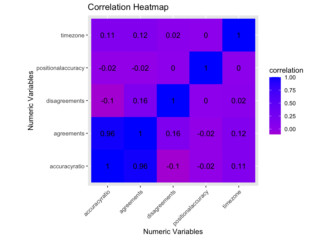
After creating the correlation heatmap comparing my numeric variables (these include: id agreements, id disagreements, overall accuracy of identification, positional accuracy, and time zone/location estimate), it appears there is no strong correlation between any of the variables. My initial questions of relation between id accuracy ratio and location (timezone) and the relationship between disagreements and positional accuracy could be answered with this data in that there is little to no relationship between these variables.
Number of Disagreements by Positional Accuracy and faceted Location (timezone estimate)
ggplot(idbugs2, aes(disagreements, positionalaccuracy)) +
  geom_point(aes(color=taxon_family_name)) +
  ggtitle("Number of Disagreements by Positional Accuracy and faceted Location (timezone)")+
  xlab("Number of Disagreements in ID") + ylab("Positional Accuracy") + facet_wrap( ~ timezone2 ) +
  theme(legend.position = "none")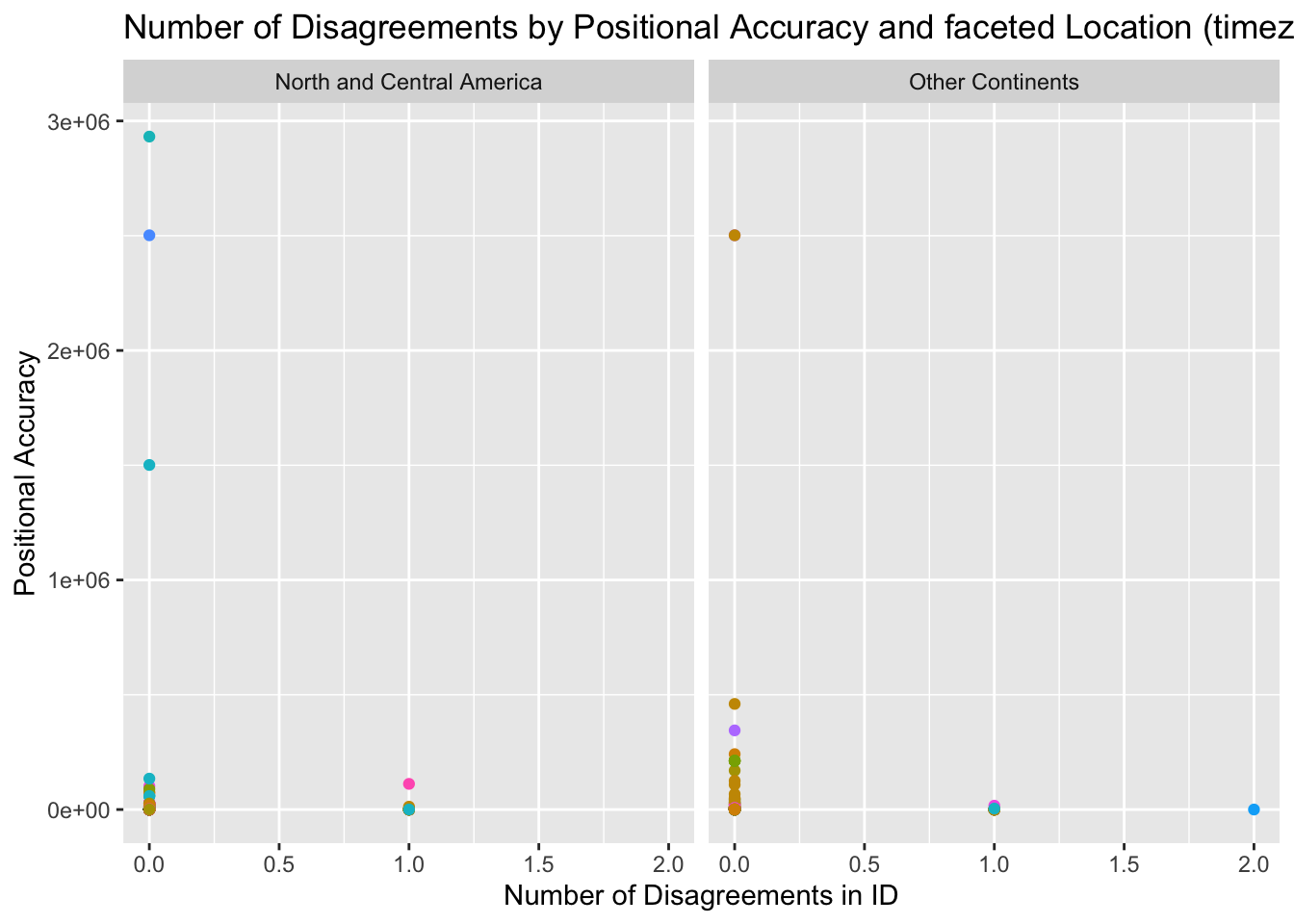
After creating this scatterplot that compares positional accuracy and number of disagreements while faceting by location (time zone estimate), not much information can be drawn from the results. It appears that most of the data has zero disagreements no matter the positional accuracy rating. In addition, there seems to be a slightly higher range in the number of disagreements among observations from non-North American continents while there is a higher range in positional accuracy. These discrepancies could be attributed to outliers.
Agreements and Disagreements by Location (timezone estimate)
ggplot(idbugs2, aes(x = disagreements, y = agreements, fill=timezone2))+
  geom_bar(stat="summary",fun.y="mean", position="dodge")+
  geom_errorbar(stat="summary",position="dodge") +
  ggtitle("Agreements and Disagreements by Location (timezone estimate)") +
  xlab("Number of Disagreements") + ylab("Number of Agreements") + scale_y_continuous(breaks=seq(0, 5, 1)) + scale_x_continuous(breaks=seq(0,2,1))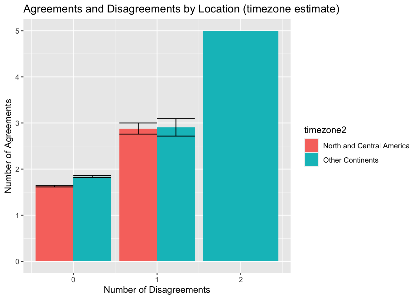
After creating this bar chart which compares the number of disagreements and agreements in identification between locations (time zone estimates), a few trends can be observed. It appears that observations outside of North and Central America have higher mean agreements and disagreements overall. Other continents are the only location group to have a mean of 2 disagreements and a mean of more than 5 agreements. This suggests that there is more identification discussion amongst groups from outside of North America.
Dimensionality Reduction using PCA
For this dataset, it was a better idea to use PAM clustering with gower as some of the most important variables in this dataset are categorical (Family, Genus, Species, Location (timezone2)). The following are the steps and code used to create this clustering.
Using gower to implement categorical variables in the clustering of the data.
Converting useful categorical variables into factor to allow for clustering
idbugs3<-idbugs2 %>%
  select(-id,-time_zone,-observed_on,-description, -quality_grade, -captive_cultivated, -place_guess, -coordinates, -species_guess, -scientific_name, -common_name, -timezone, -num_identification_agreements1, -num_identification_disagreements1) %>%
  mutate_if(is.character,as.factor)
Creating clusters using gower
gower1<-daisy(idbugs3,metric="gower") %>% scaleCreating a silhouette plot to determine how many clusters should be used with pam
sil_width<-vector()
for(i in 2:10){
pam_fit <- pam(gower1, diss = TRUE, k = i)
sil_width[i] <- pam_fit$silinfo$avg.width
}
ggplot()+geom_line(aes(x=1:10,y=sil_width))+scale_x_continuous(name="k",breaks=1:10)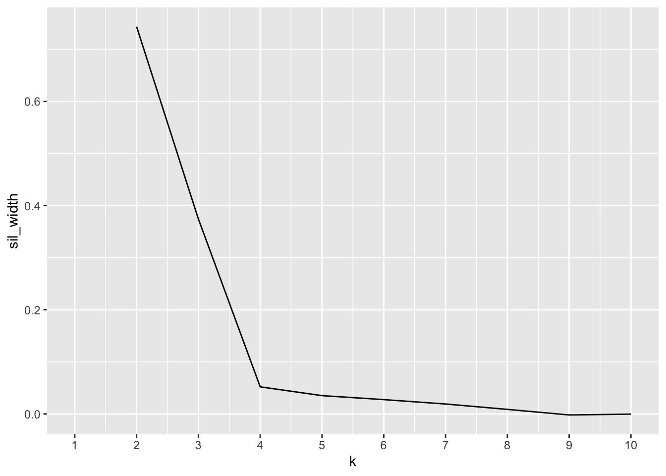 After looking at the plot, it appears the most useful number of clusters is 2 clusters as it has the highest peak on the plot.
Creating 2 clusters using PAM
pam1<-pam(gower1,k=2,diss=T)
pam_idbugs<-idbugs3%>%mutate(cluster=as.factor(pam1$clustering))
View of clusters
table<-pam_idbugs%>%group_by(timezone2)%>%count(cluster)%>%arrange(desc(n))%>%
pivot_wider(names_from="cluster",values_from="n",values_fill = list('n'=0))
table
## # A tibble: 2 x 3
## # Groups: timezone2 [2]
## timezone2 `2` `1`
## <fct> <int> <int>
## 1 North and Central America 1869 214
## 2 Other Continents 428 1432Clusters fit well for time zone
GGpairs was not compatible with my data so I created two plots which compare my cluster accuracy amongst my numeric variables**
ggplot(pam_idbugs, aes(x=positionalaccuracy,y=disagreements, color=cluster))+
  geom_point()+
  ggtitle("Clustering by Positional Accuracy and ID Disagreements") +
  xlab("Positional Accuracy") +ylab("ID Disagreements")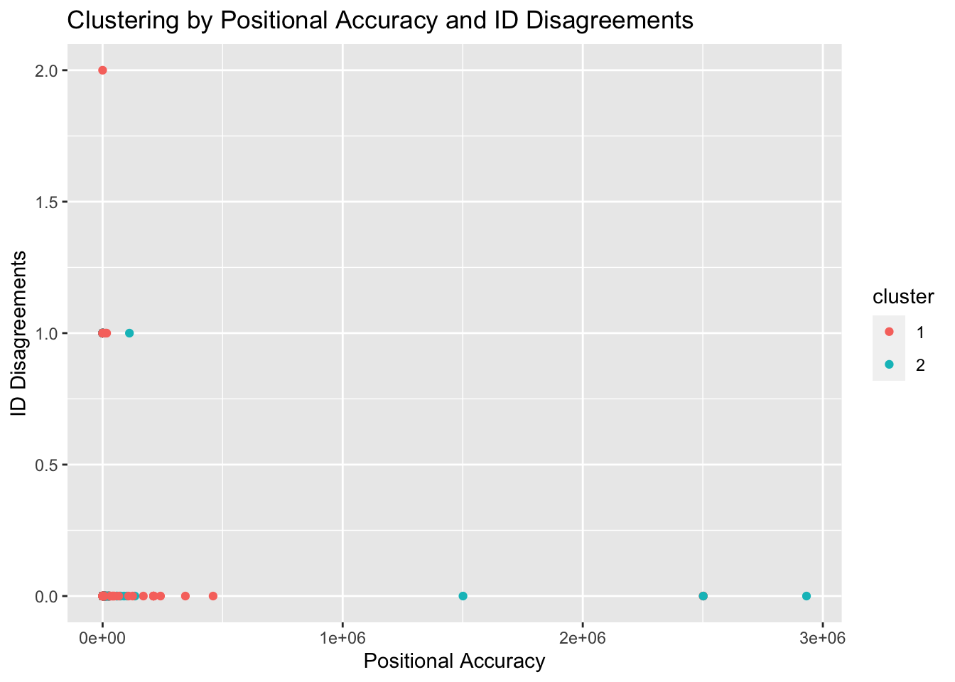
ggplot(pam_idbugs, aes(x=timezone2,y=accuracyratio, color=cluster)) +
  geom_point() +
  ggtitle("Clustering by Location (time zone estimate) and ID Accuracy Ratio") +
  xlab("Location (Time zone estimate)") + ylab("ID Accuracy Ratio")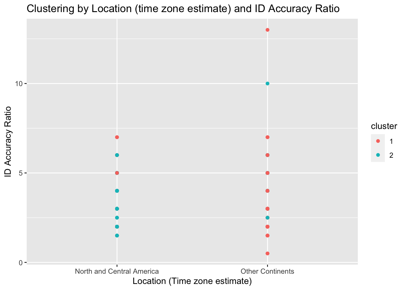
Average silhouette length
pam1$silinfo$avg.width ## [1] 0.7435828