January 1, 0001
Introduction
The dataset chosen for this project is called skulls. Skulls is a collection of measurements of ancient adult skulls found in Egypt. There are 150 skulls measured (30 from each time frame) and 5 variables. The explanatory variables include: epoch (c4000BCE, c3300BCE, c1850BCE, c200BCE, and c150CE), basibregmatic height (mm), basialiveolar length (mm), and nasal height (mm). The response variable that this project will study is maximum breath (mm).
This dataset is of interest because it could tell us how the size and proportions of skulls have changed over time in this area. I am particularly interested in how the epoch and other measurements effect the maximum breath of skulls (maximum breath is the width of skulls at the widest point of the cranium).
library(tidyverse)
library(ggplot2)
library(dplyr)

#install.packages("HSAUR")
library(HSAUR)
skulls<-skulls
head(skulls)
## epoch mb bh bl nh
## 1 c4000BC 131 138 89 49
## 2 c4000BC 125 131 92 48
## 3 c4000BC 131 132 99 50
## 4 c4000BC 119 132 96 44
## 5 c4000BC 136 143 100 54
## 6 c4000BC 138 137 89 56str(skulls)## 'data.frame': 150 obs. of 5 variables:
## $ epoch: Ord.factor w/ 5 levels "c4000BC"<"c3300BC"<..:
1 1 1 1 1 1 1 1 1 1 ...
## $ mb : num 131 125 131 119 136 138 139 125 131 134 ...
## $ bh : num 138 131 132 132 143 137 130 136 134 134 ...
## $ bl : num 89 92 99 96 100 89 108 93 102 99 ...
## $ nh : num 49 48 50 44 54 56 48 48 51 51 ...#I am going to add 2 additional variables to the dataset in order to separate the Epoch variable into the BCE and CE time periods. This will be useful for a later part of the project.
skulls2<-skulls %>% mutate(timenum=ifelse(epoch=="cAD150",1,0), timechar=ifelse(epoch=="cAD150", "CE", "BCE"))
#A view of the edited dataset
head(skulls2)## epoch mb bh bl nh timenum timechar
## 1 c4000BC 131 138 89 49 0 BCE
## 2 c4000BC 125 131 92 48 0 BCE
## 3 c4000BC 131 132 99 50 0 BCE
## 4 c4000BC 119 132 96 44 0 BCE
## 5 c4000BC 136 143 100 54 0 BCE
## 6 c4000BC 138 137 89 56 0 BCEstr(skulls2)## 'data.frame': 150 obs. of 7 variables:
## $ epoch : Ord.factor w/ 5 levels "c4000BC"<"c3300BC"<..:
1 1 1 1 1 1 1 1 1 1 ...
## $ mb : num 131 125 131 119 136 138 139 125 131 134 ...
## $ bh : num 138 131 132 132 143 137 130 136 134 134 ...
## $ bl : num 89 92 99 96 100 89 108 93 102 99 ...
## $ nh : num 49 48 50 44 54 56 48 48 51 51 ...
## $ timenum : num 0 0 0 0 0 0 0 0 0 0 ...
## $ timechar: chr "BCE" "BCE" "BCE" "BCE" ...MANOVA
Hypotheses:
- H0: For all the numeric variables (maximum breath (mm), basibregmatic height (mm), basialiveolar length (mm), and nasal height (mm)), means for each epoch are equal.
- HA: For all the numeric variables (maximum breath (mm), basibregmatic height (mm), basialiveolar length (mm), and nasal height (mm)), means for each epoch are not equal.
Assumptions
#- We assume this is a random sample with independent observations
# Multivariate normality of DVs (or each group )

library(mvtnorm)
library(ggExtra)

ggplot(skulls, aes(x = mb, y = bh, fill=epoch)) +
  geom_point(alpha = .5) +
  geom_density_2d(h=15) +
  coord_fixed() +
  facet_wrap(~epoch) +
  ggtitle("Density Plot of Maximum Breath and Basibregmatic Height by Epoch")+
  xlab("Maximum Breath (mm)") +ylab("Basibregmatic Height (mm)")
ggplot(skulls, aes(x = mb, y = bl, fill=epoch)) +
  geom_point(alpha = .5) +
  geom_density_2d(h=15) +
  coord_fixed() +
  facet_wrap(~epoch) +
  ggtitle("Density Plot of Maximum Breath and Basialiveolar Length by Epoch")+
  xlab("Maximum Breath (mm)") +ylab("Basialiveolar Length (mm)")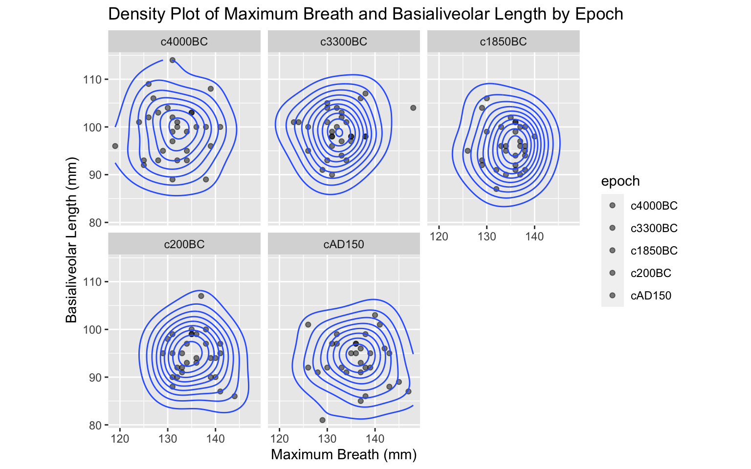
ggplot(skulls, aes(x = mb, y = nh, fill=epoch)) +
  geom_point(alpha = .5) +
  geom_density_2d(h=15) +
  coord_fixed() +
  facet_wrap(~epoch) +
  ggtitle("Density Plot of Maximum Breath and Nasal Height by Epoch")+
  xlab("Maximum Breath (mm)") +ylab("Nasal Height (mm)")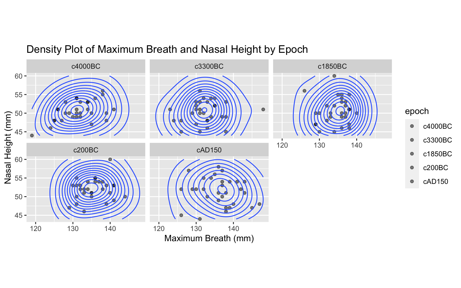
ggplot(skulls, aes(x = bh, y = bl, fill=epoch)) +
  geom_point(alpha = .5) +
  geom_density_2d(h=15) +
  coord_fixed() +
  facet_wrap(~epoch) +
  ggtitle("Density Plot of Basibregmatic Height and Basialiveolar Length by Epoch")+
  xlab("Basibregmatic Height (mm)") + ylab("Basialiveolar Length (mm)")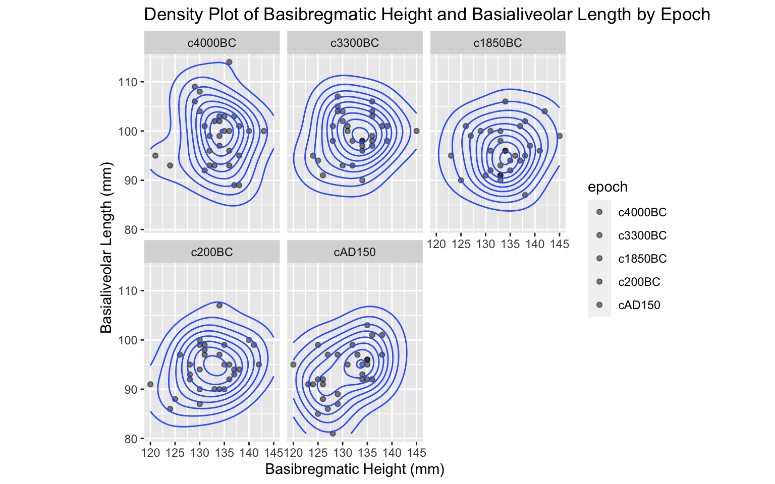
ggplot(skulls, aes(x = bh, y = nh, fill=epoch)) +
  geom_point(alpha = .5) +
  geom_density_2d(h=15) +
  coord_fixed() +
  facet_wrap(~epoch) +
  ggtitle("Density Plot of Basibregmatic Height and Nasal Height by Epoch")+
  xlab("Basibregmatic Height (mm)") +ylab("Nasal Height (mm)")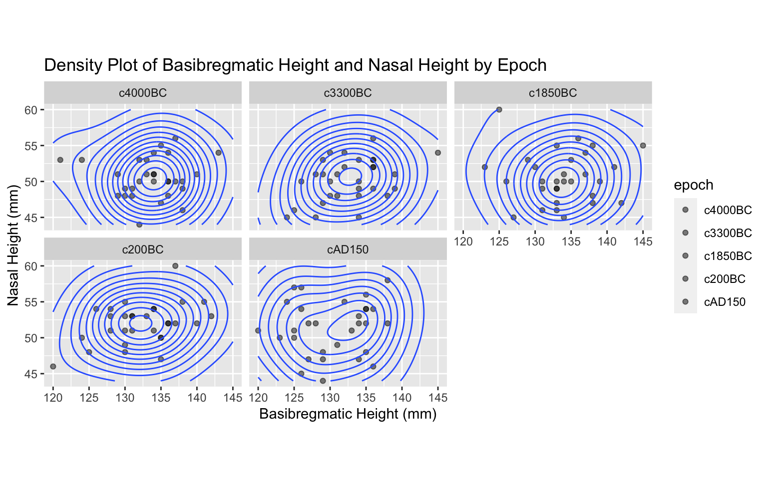
ggplot(skulls, aes(x = bl, y = nh, fill=epoch)) +
  geom_point(alpha = .5) +
  geom_density_2d(h=15) +
  coord_fixed() +
  facet_wrap(~epoch) +
  ggtitle("Density Plot of Basibregmatic Height and Basialiveolar Length by Epoch")+
xlab("Basialiveolar Length (mm)") +ylab("Nasal Height (mm)") 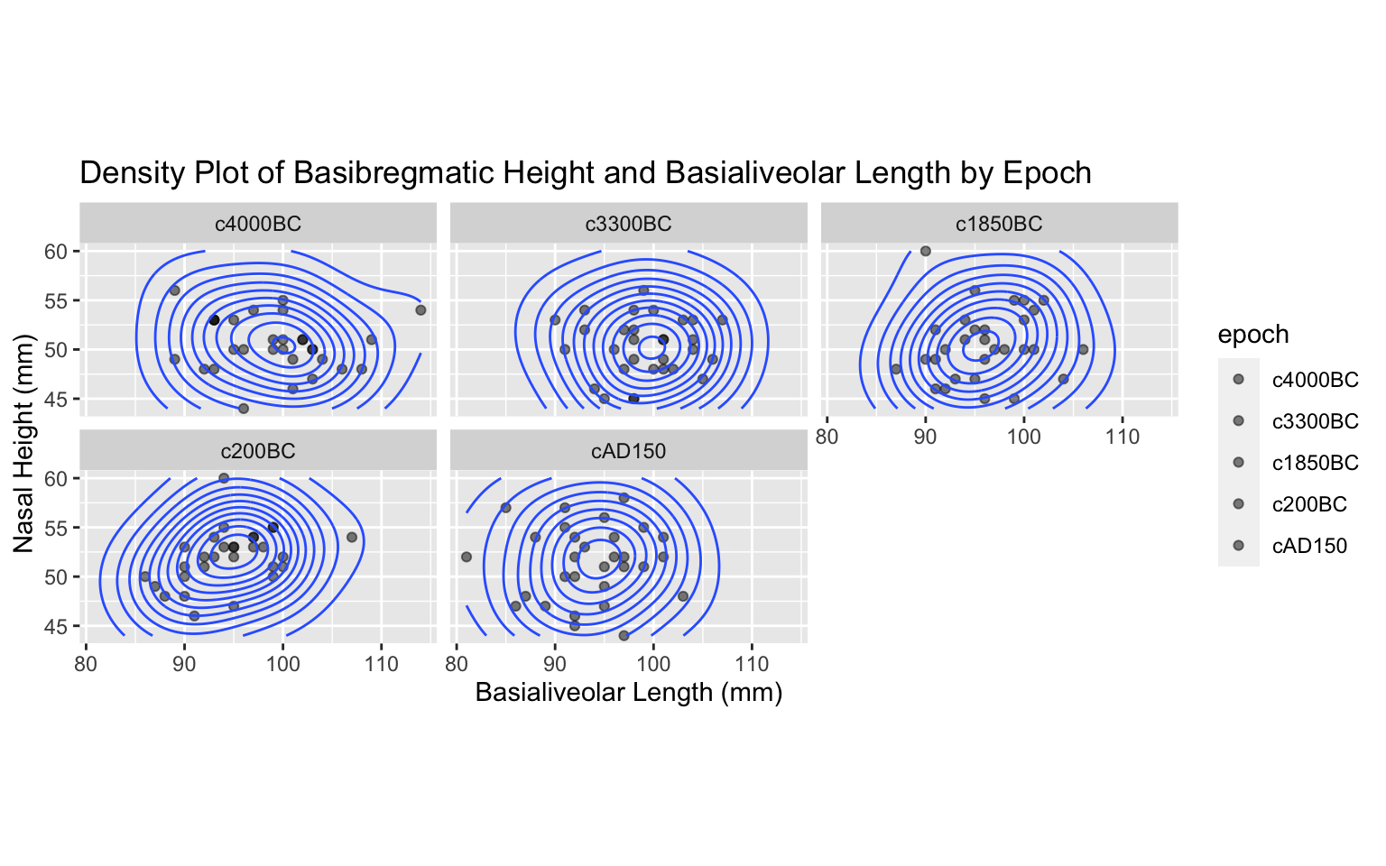
#Our dataset appears to have a very loose multivariate normality.

#- Homogeneity of within-group covariance matrices

covmats1<-skulls%>%group_by(epoch)%>%do(covs=cov(.[2:5]))
for(i in 1:5){print(as.character(covmats1$epoch[i])); print(covmats1$covs[i])}
## [1] "c4000BC"
## [[1]]
## mb bh bl nh
## mb 26.309195 4.1517241 0.4540230 7.2459770
## bh 4.151724 19.9724138 -0.7931034 0.3931034
## bl 0.454023 -0.7931034 34.6264368 -1.9195402
## nh 7.245977 0.3931034 -1.9195402 7.6367816
##
## [1] "c3300BC"
## [[1]]
## mb bh bl nh
## mb 23.136782 1.010345 4.7678161 1.8425287
## bh 1.010345 21.596552 3.3655172 5.6241379
## bl 4.767816 3.365517 18.8919540 0.1908046
## nh 1.842529 5.624138 0.1908046 8.7367816
##
## [1] "c1850BC"
## [[1]]
## mb bh bl nh
## mb 12.1195402 0.78620690 -0.7747126 0.89885057
## bh 0.7862069 24.78620690 3.5931034 -0.08965517
## bl -0.7747126 3.59310345 20.7229885 1.67011494
## nh 0.8988506 -0.08965517 1.6701149 12.59885057
##
## [1] "c200BC"
## [[1]]
## mb bh bl nh
## mb 15.362069 -5.534483 -2.172414 2.051724
## bh -5.534483 26.355172 8.110345 6.148276
## bl -2.172414 8.110345 21.085057 5.328736
## nh 2.051724 6.148276 5.328736 7.964368
##
## [1] "cAD150"
## [[1]]
## mb bh bl nh
## mb 28.6264368 -0.2298851 -1.8793103 -1.9942529
## bh -0.2298851 24.7126437 11.7241379 2.1494253
## bl -1.8793103 11.7241379 25.5689655 0.3965517
## nh -1.9942529 2.1494253 0.3965517 13.8264368#The covariances aren't perfect, and do not truly meet this assumption.
#The test will be continued despite this.
#- No Outliers & Linear relationships among DVs
#Outliers visual test
ggplot(skulls, aes(x = mb, y = bh, fill=epoch)) +
geom_point() +
ggtitle("Scatter Plot of Maximum Breath and Basibregmatic Height by Epoch")+
xlab("Maximum Breath (mm)") +ylab("Basibregmatic Height (mm)")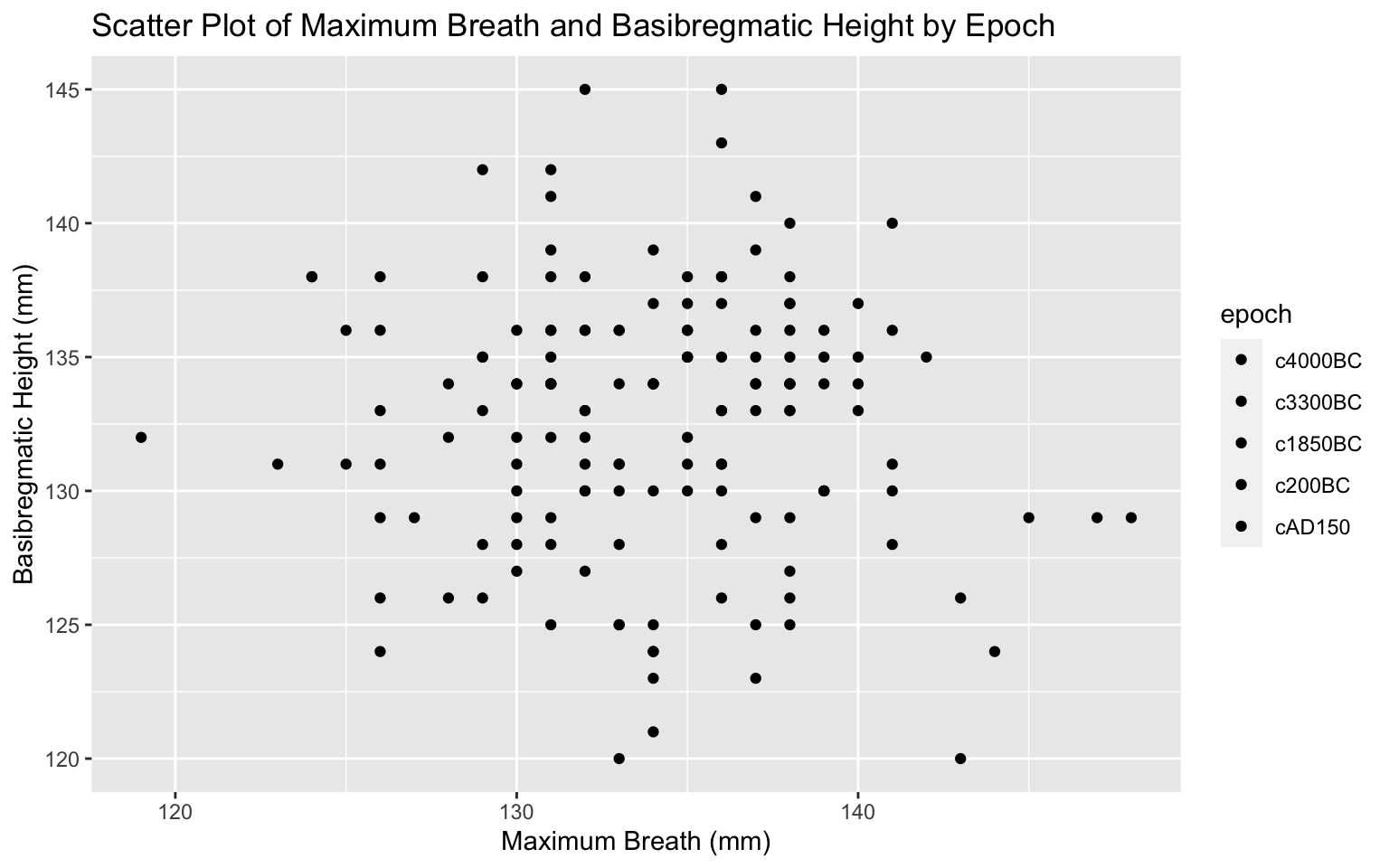
ggplot(skulls, aes(x = mb, y = bl, fill=epoch)) +
  geom_point() +
  ggtitle("Scatter Plot of Maximum Breath and Basialiveolar Length by Epoch")+
  xlab("Maximum Breath (mm)") +ylab("Basialiveolar Length (mm)")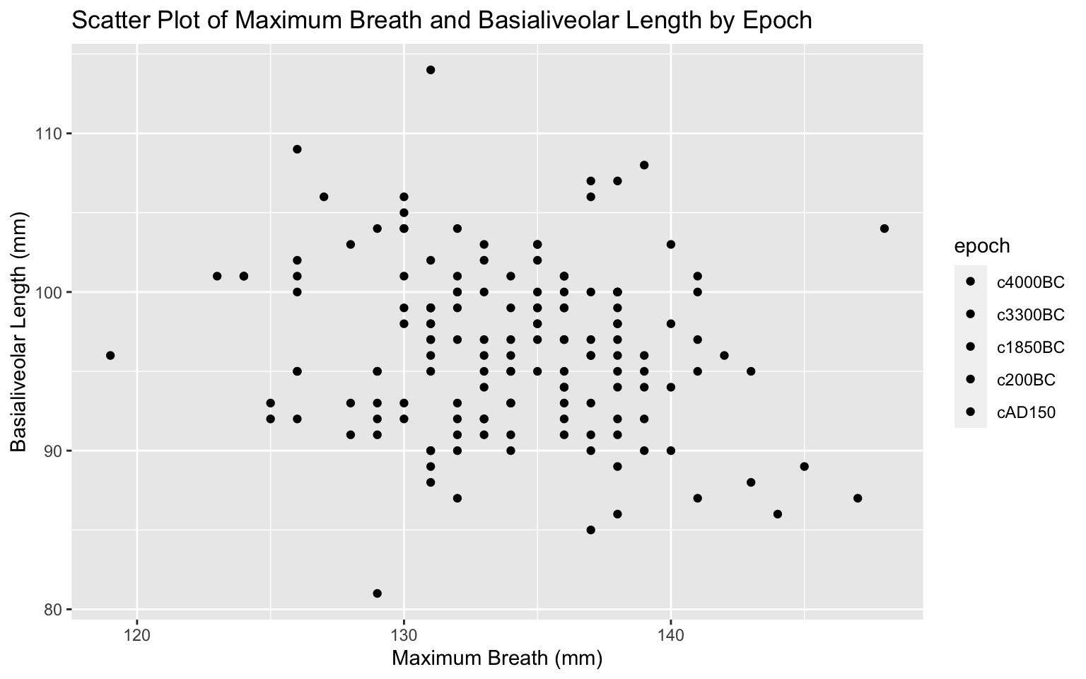
ggplot(skulls, aes(x = mb, y = nh, fill=epoch)) +
  geom_point() +
  ggtitle("Scatter Plot of Maximum Breath and Nasal Height by Epoch")+
  xlab("Maximum Breath (mm)") +ylab("Nasal Height (mm)")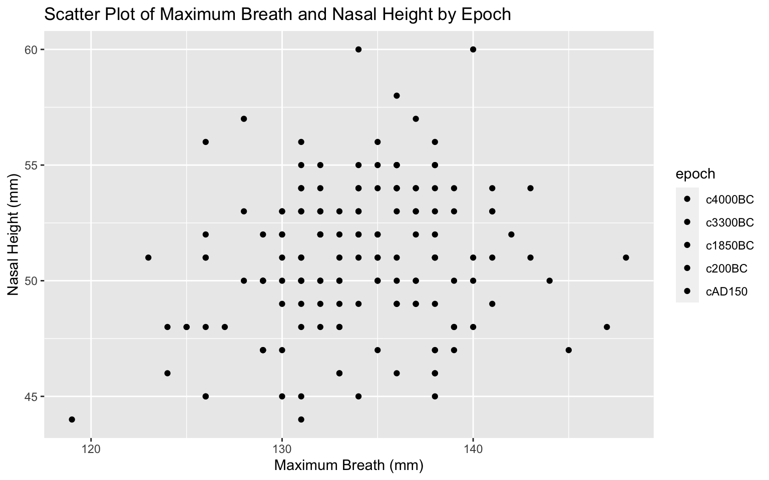
ggplot(skulls, aes(x = bh, y = bl, fill=epoch)) +
  geom_point() +
  ggtitle("Scatter Plot of Basibregmatic Height and Basialiveolar Length by Epoch")+
  xlab("Basibregmatic Height (mm)") + ylab("Basialiveolar Length (mm)")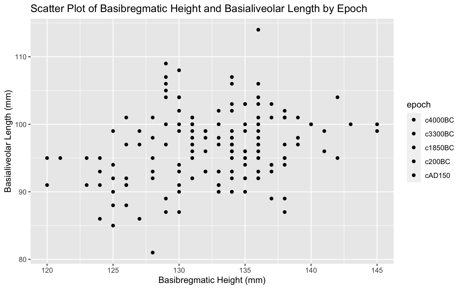
ggplot(skulls, aes(x = bh, y = nh, fill=epoch)) +
  geom_point()+
  ggtitle("Scatter Plot of Basibregmatic Height and Nasal Height by Epoch")+
  xlab("Basibregmatic Height (mm)") +ylab("Nasal Height (mm)")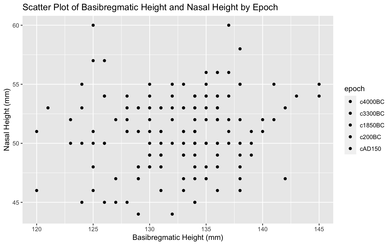
ggplot(skulls, aes(x = bl, y = nh, fill=epoch)) +
  geom_point() +
  ggtitle("Scatter Plot of Basibregmatic Height and Basialiveolar Length by Epoch")+
  xlab("Basialiveolar Length (mm)") +ylab("Nasal Height (mm)")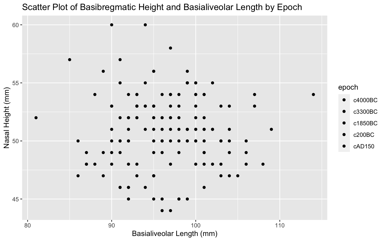
#There don't appear to be any outliers

#From the graphs above, there doesn't seem to be a linear relationship between any of the variables.

#Checking linear relationship
cor_skulls <- skulls %>% select_if(is.numeric) %>% cor

library(kableExtra)

cor_skulls %>% kable() %>%
kable_styling(bootstrap_options = c("striped", "hover", "condensed"))| mb | bh | bl | nh | |
|---|---|---|---|---|
| mb | 1.0000000 | -0.0619037 | -0.1569728 | 0.1825475 |
| bh | -0.0619037 | 1.0000000 | 0.2643529 | 0.1467508 |
| bl | -0.1569728 | 0.2643529 | 1.0000000 | -0.0063801 |
| nh | 0.1825475 | 0.1467508 | -0.0063801 | 1.0000000 |
#None of the variables share a strong linear relationship with each other.
#This assumption is not met.
#This also makes it seem that the No multicollinearity assumption is met
#because none of the DVs are too linearly correlated.
For the most part, the assumptions were not met. However, the show must go on.
MANOVA
man1<-manova(cbind(mb,bh,bl,nh)~epoch, data=skulls)
summary(man1)
## Df Pillai approx F num Df den Df Pr(>F)
## epoch 4 0.35331 3.512 16 580 4.675e-06 ***
## Residuals 145
## ---
## Signif. codes: 0 '***' 0.001 '**' 0.01 '*' 0.05 '.' 0.1
' ' 1#MANOVA test is significant with a p value of 4.675e-06
#Univariate ANOVAs and pairwise t-tests must be conductedUnivariate ANOVAs
summary.aov(man1)## Response mb :
## Df Sum Sq Mean Sq F value Pr(>F)
## epoch 4 502.83 125.707 5.9546 0.0001826 ***
## Residuals 145 3061.07 21.111
## ---
## Signif. codes: 0 '***' 0.001 '**' 0.01 '*' 0.05 '.' 0.1
' ' 1
##
## Response bh :
## Df Sum Sq Mean Sq F value Pr(>F)
## epoch 4 229.9 57.477 2.4474 0.04897 *
## Residuals 145 3405.3 23.485
## ---
## Signif. codes: 0 '***' 0.001 '**' 0.01 '*' 0.05 '.' 0.1
' ' 1
##
## Response bl :
## Df Sum Sq Mean Sq F value Pr(>F)
## epoch 4 803.3 200.823 8.3057 4.636e-06 ***
## Residuals 145 3506.0 24.179
## ---
## Signif. codes: 0 '***' 0.001 '**' 0.01 '*' 0.05 '.' 0.1
' ' 1
##
## Response nh :
## Df Sum Sq Mean Sq F value Pr(>F)
## epoch 4 61.2 15.300 1.507 0.2032
## Residuals 145 1472.1 10.153skulls%>%group_by(epoch)%>%summarize(mean(mb),mean(bh), mean(bl), mean(nh))## # A tibble: 5 x 5
## epoch `mean(mb)` `mean(bh)` `mean(bl)` `mean(nh)`
## <ord> <dbl> <dbl> <dbl> <dbl>
## 1 c4000BC 131. 134. 99.2 50.5
## 2 c3300BC 132. 133. 99.1 50.2
## 3 c1850BC 134. 134. 96.0 50.6
## 4 c200BC 136. 132. 94.5 52.0
## 5 cAD150 136. 130. 93.5 51.4#The maximum breath, basibregmatic height, and basialiveolar length variables all show a significant mean
#difference in one or more of the epochs. The pairwise t-tests will give more insight on which epochs show the
#most difference.Pairwise t-tests
pairwise.t.test(skulls$mb,skulls$epoch,
                p.adj="none")
##
## Pairwise comparisons using t tests with pooled SD
##
## data: skulls$mb and skulls$epoch
##
## c4000BC c3300BC c1850BC c200BC
## c3300BC 0.40065 - - -
## c1850BC 0.00992 0.07880 - -
## c200BC 0.00065 0.00917 0.38518 -
## cAD150 8.4e-05 0.00167 0.15401 0.57501
##
## P value adjustment method: nonepairwise.t.test(skulls$bh,skulls$epoch,
p.adj="none")##
## Pairwise comparisons using t tests with pooled SD
##
## data: skulls$bh and skulls$epoch
##
## c4000BC c3300BC c1850BC c200BC
## c3300BC 0.4731 - - -
## c1850BC 0.8732 0.3808 - -
## c200BC 0.3006 0.7497 0.2326 -
## cAD150 0.0100 0.0606 0.0063 0.1182
##
## P value adjustment method: nonepairwise.t.test(skulls$bl,skulls$epoch,
p.adj="none")##
## Pairwise comparisons using t tests with pooled SD
##
## data: skulls$bl and skulls$epoch
##
## c4000BC c3300BC c1850BC c200BC
## c3300BC 0.93733 - - -
## c1850BC 0.01475 0.01817 - -
## c200BC 0.00037 0.00048 0.23936 -
## cAD150 1.6e-05 2.2e-05 0.04788 0.41704
##
## P value adjustment method: nonepairwise.t.test(skulls$nh,skulls$epoch,
p.adj="none")##
## Pairwise comparisons using t tests with pooled SD
##
## data: skulls$nh and skulls$epoch
##
## c4000BC c3300BC c1850BC c200BC
## c3300BC 0.716 - - -
## c1850BC 0.968 0.686 - -
## c200BC 0.084 0.037 0.091 -
## cAD150 0.313 0.170 0.332 0.467
##
## P value adjustment method: noneError rate & Bonferroni Correction
#1 MANOVA
#4 ANOVAs
#20 t-tests
1+4+20
## [1] 25#25 total tests
#Error rate
1-(.95)^25## [1] 0.7226104#Bonferroni Correction
.05/25## [1] 0.002Visualiation
skulls %>% select(epoch,mb,bh,bl, nh) %>%
  pivot_longer(-1,names_to='DV', values_to='measurement') %>%
  ggplot(aes(epoch,measurement,fill=epoch)) +
  geom_bar(stat="summary") +
  geom_errorbar(stat="summary", width=.5) +
  facet_wrap(~DV, nrow=2) +
  coord_flip() +
  ylab("") +
  theme(legend.position = "none")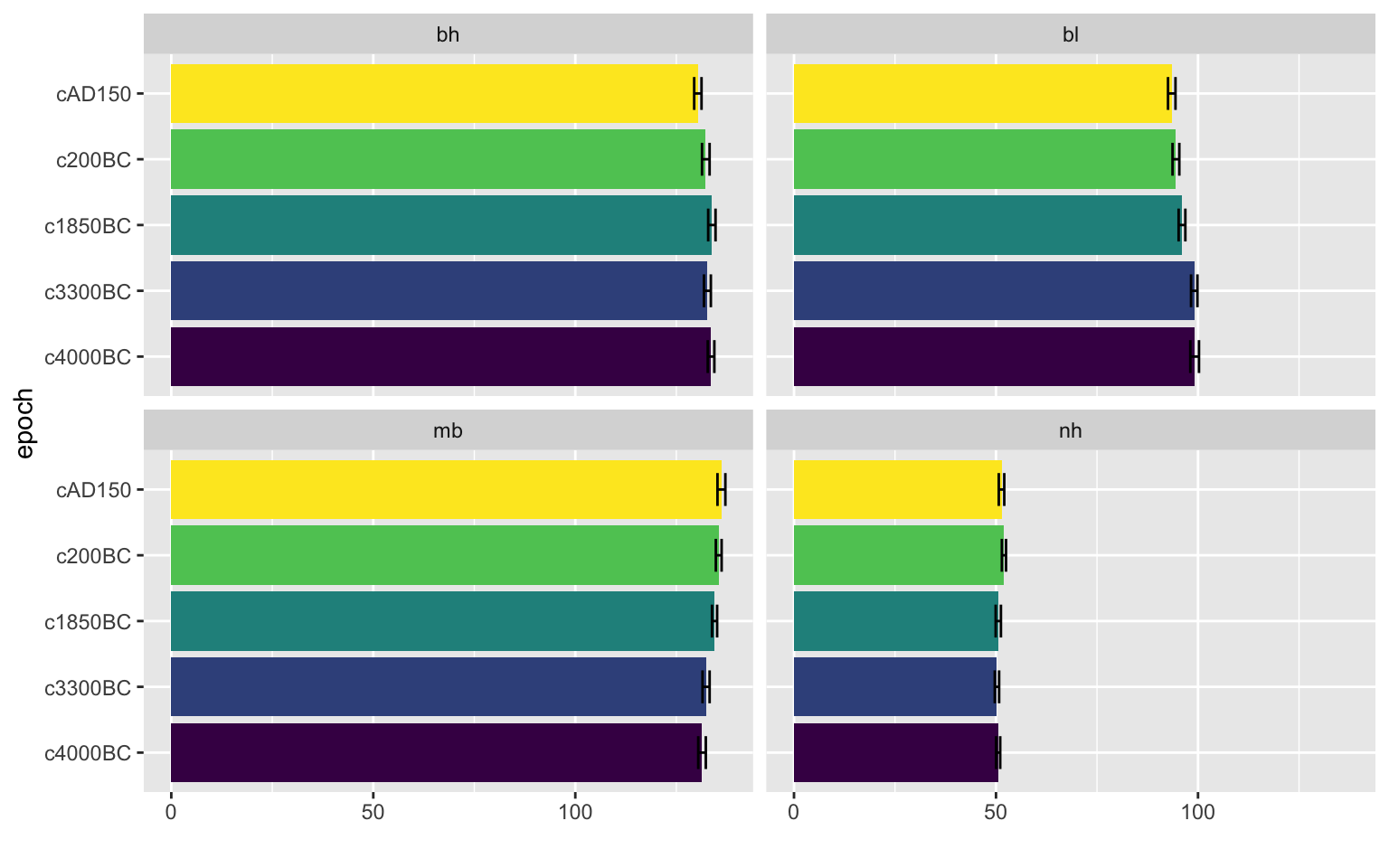
Conclusions Drawn from MANOVA
A one-way MANOVA was conducted to determine the effect of the time period (epochs: c4000BCE, c3300BCE, c1850BCE, c200BCE, and c150CE) on 4 dependent variables (maximum breath (mm), basibregmatic height (mm), basialiveolar length (mm), and nasal height (mm)) The bivariate density plots for each group do not fully follow multivariate normality. The assumption of in-group homogeneity was tested using covariance matrices and was not met. Bivariate linearity assumptions were also not met after consulting individual scatterplots and the correlation matrix. No univariate or multivariate outliers were evident. The MANOVA test was ill-advised, but continued nonetheless.
Significant differences were found among the epochs for at least one of the dependent variables (Pillai=0.35331, approx. f=3.512, p-value=4.675e-06), further univariate ANOVAS and pairwise t-tests were conducted to determine which of the response variables and epochs differed.
Univariate ANOVAs were conducted, The univariate ANOVAs for maximum breath (F=5.9546, p-value=0.0001826) and basialiveolar length (F=8.3057, p-value=4.636e-06) were significant after the Bonferroni corrected level of significance (alpha=.002). From this point forward, the Bonferroni correction will be used because the type one error rate is 72.26% otherwise.
Pairwise t-tests were performed as post-hoc analyses to determine which epochs showed differences across the response variables. The 4000BCE epoch differed significantly with 200BCE (p-value=0.00065) and AD150 (p-value= 4e-05). The 3300BCE epoch also differed significantly with the AD150 epoch for maximum breath (p-value=0.00167). The 4000BCE epoch differed significantly from the 200BCE (p-value= 0.00037) and AD150 (p-value= 1.6e-05) epochs for basialiveolar length and the 3000BCE epoch differed with these as well (p-values= 0.00048 and 2.2e-05 respectfully).
If the assumptions were met, this would give enough evidence to reject the null hypothesis that all the numeric variables (maximum breath (mm), basibregmatic height (mm), basialiveolar length (mm), and nasal height (mm)), means for each epoch are equal. This set of tests gives insight into which variables and epochs differ significantly. It appears that the maximum breath and basialiveolar length variables changed the most over time and that the differences are greatest between the oldest (4000BCE & 3300BCE) and youngest (200BCE & AD150) epochs.
Randomiation test (Mean Difference)
For this section of the project, a randomization test will be conducted. Since the variables of interest are epoch (categorical) and maximum breath (numeric), a mean difference test will be used.
Hypotheses:
H0: Mean maximum breath is the same across all epochs HA: Mean maximum breath is different in one or more epochs
Visualization of original sample:
ggplot(skulls2,aes(mb,fill=timechar))+
  geom_histogram()+
  facet_wrap(~timechar)+
  theme(legend.position="none")+
  ggtitle("Histogram of Maximum Breath by Time")+
  xlab("Maximum Breath (mm)")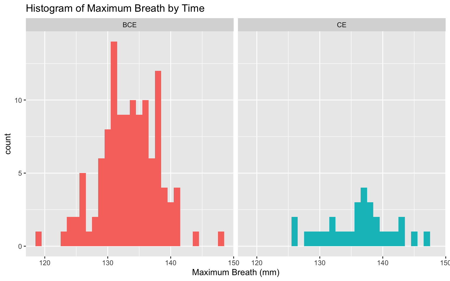
Randomization Test
#Original mean difference
origdiff<-skulls2%>%group_by(timechar)%>%
  summarize(means=mean(mb))%>%
  summarize(`mean_diff:`=diff(means))
origdiff
## # A tibble: 1 x 1
## `mean_diff:`
## <dbl>
## 1 2.74#Random distribution
random_dist<-vector()
for(i in 1:5000){
sample_<-data.frame(mb=sample(skulls2$mb),timechar=skulls2$timechar)
random_dist[i]<-mean(sample_[sample_$timechar=="CE",]$mb)-
mean(sample_[sample_$timechar=="BCE",]$mb)}
#Visualization of the sample mean difference compared to the random distribution created above.
{hist(random_dist,main="",ylab=""); abline(v = 2.741667,col="red")}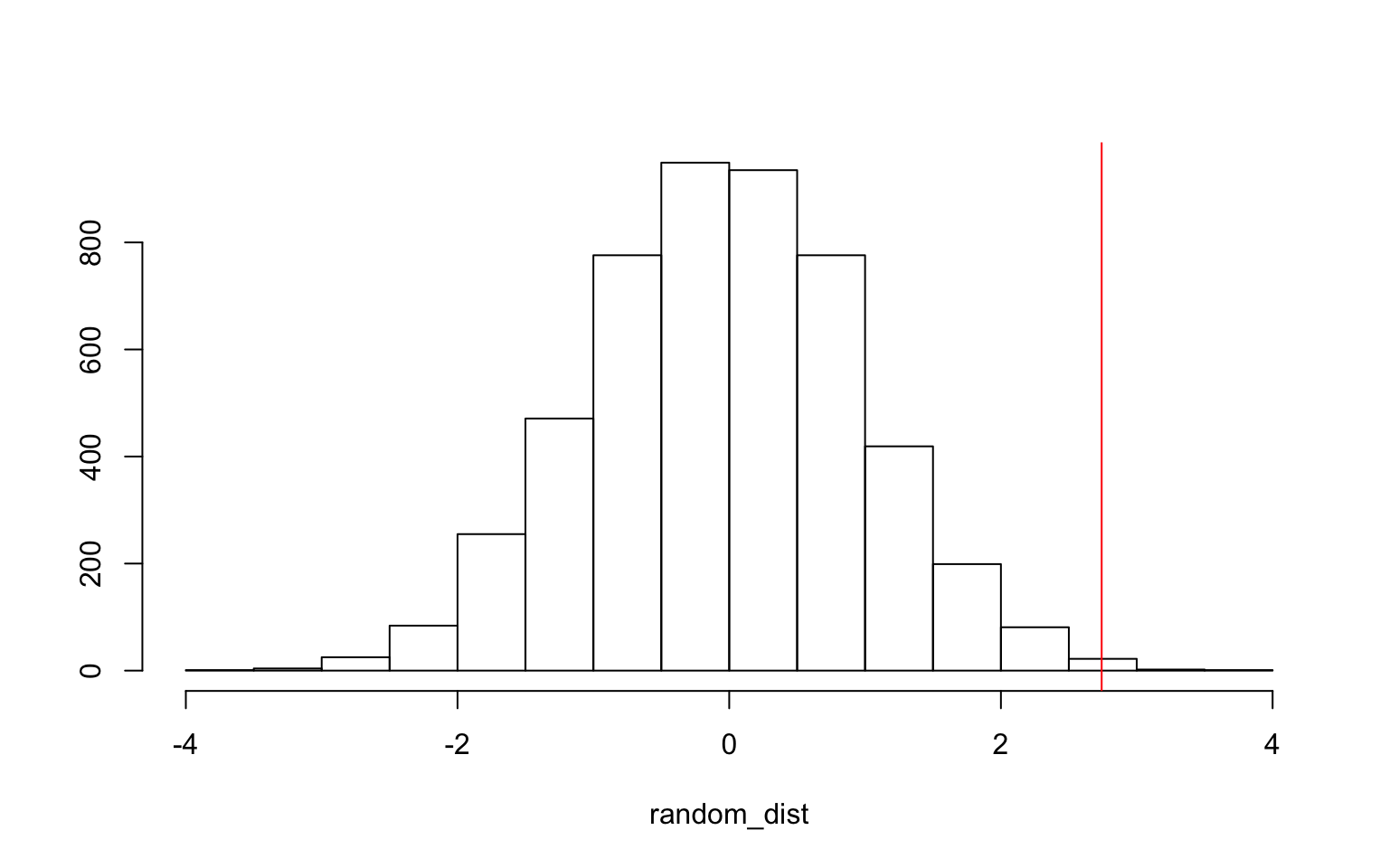
##This seems like an significant difference.

#Calculating the p-value for the likelihood that once could get this result by chance.
mean(random_dist>2.741667 | random_dist< -2.741667)
## [1] 0.004##That is a very small p-value.Conclusions drawn from Randomization test
After creating a random distribution for the difference in mean maximum breath of skulls from BCE and CE, an average mean difference of 2.741667 and a p-value of .0036 was calculated. This indicates that there is a significant difference in mean maximum breath of Egyptian skulls from BCE time periods and CE time periods.
Linear Regression Model
Hypotheses
- H01:While controlling for basibregmatic height, basialiveolar length, and nasal height, time (BCE or CE) does not explain variation in maximum breath of Egyptian skulls.
- H02:While controlling for time (BCE or CE), basialiveolar length, and nasal height, basibregmatic height, does not explain variation in maximum breath of Egyptian skulls.
- H03:While controlling for time (BCE or CE), basibregmatic height, and nasal height, basialiveolar length, does not explain variation in maximum breath of Egyptian skulls.
- H04:While controlling for time (BCE or CE), basibregmatic height, and basialiveolar length, nasal height, does not explain variation in maximum breath of Egyptian skulls.
Mean-centering numeric variables
skulls2<- skulls2 %>% mutate(mb_c=skulls2$mb-mean(skulls2$mb),
                             bh_c=skulls2$bh-mean(skulls2$bh),
                             bl_c=skulls2$bl-mean(skulls2$bl),
                             nh_c=skulls2$nh-mean(skulls2$nh))
Assumptions
#Linear Association between maximum breath and predictor variables

ggplot(skulls2, aes(timenum, mb)) +
  geom_point() +
  ggtitle ("Maximum Breath and Time") +
  xlab("Maximum Breath (mm)") +
  ylab("Time (0=BCE, 1=CE)")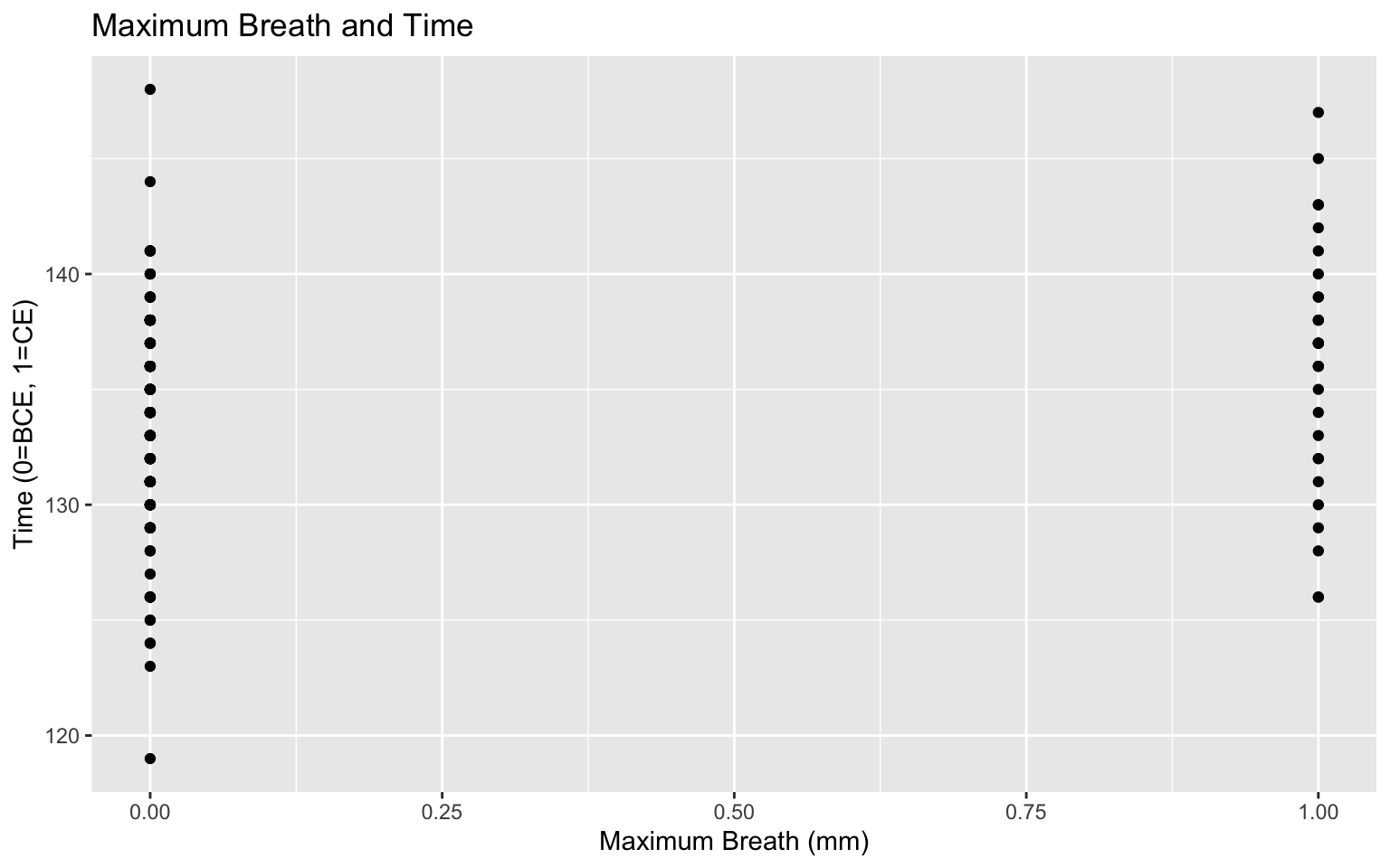
ggplot(skulls2, aes(bh_c, mb)) +
  geom_point() +
  ggtitle ("Maximum Breath and Mean-Centered Basibregmatic Height") +
  xlab("Maximum Breath (mm)") +
  ylab("Basibregmatic Height (mm)")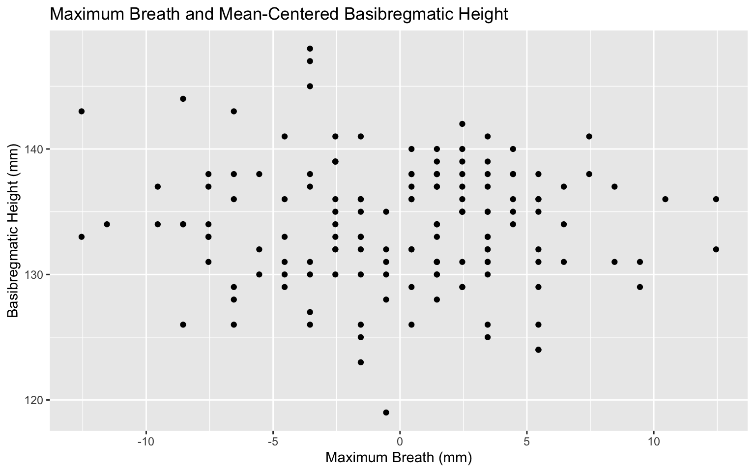
ggplot(skulls2, aes(bl_c, mb)) +
  geom_point() +
  ggtitle ("Maximum Breath and Mean-Centered Basialiveolar Length") +
  xlab("Maximum Breath (mm)") +
  ylab("Basialiveolar Length (mm)")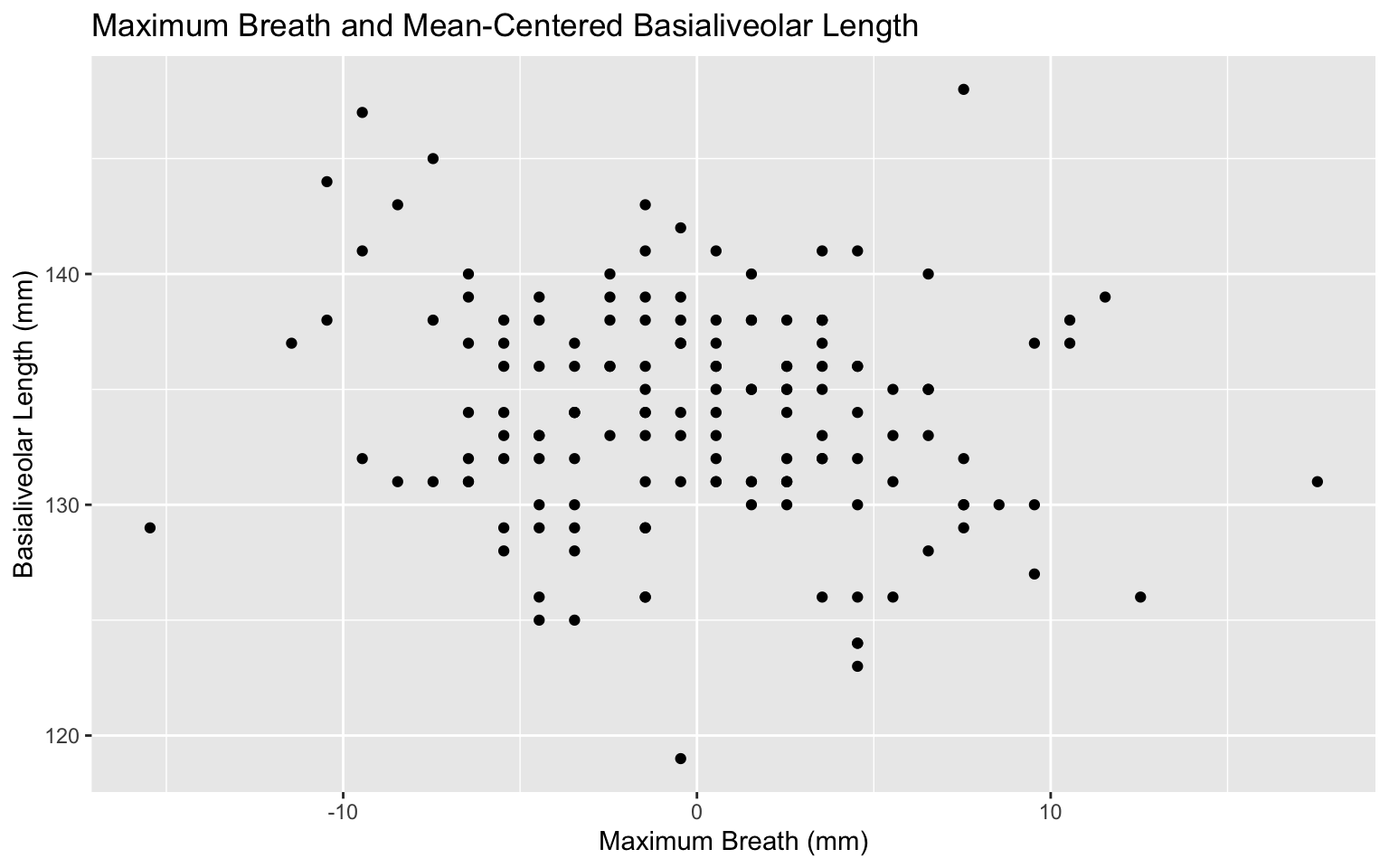
ggplot(skulls2, aes(nh_c, mb)) +
  geom_point() +
  ggtitle ("Maximum Breath and Mean-Centered Nasal Height") +
  xlab("Maximum Breath (mm)") +
  ylab("Nasal Height (mm)")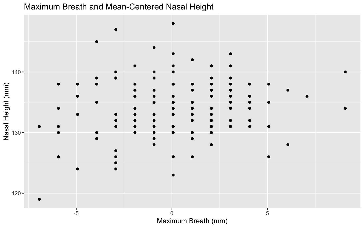
##Vague Linear Associations between explanatory variables and maximum breath.

#Normally distributed residuals
residuals<-lm(mb ~ timenum*bh_c*bl_c*nh_c, data=skulls2)$residuals
ggplot() +
  geom_histogram(aes(residuals),bins=10)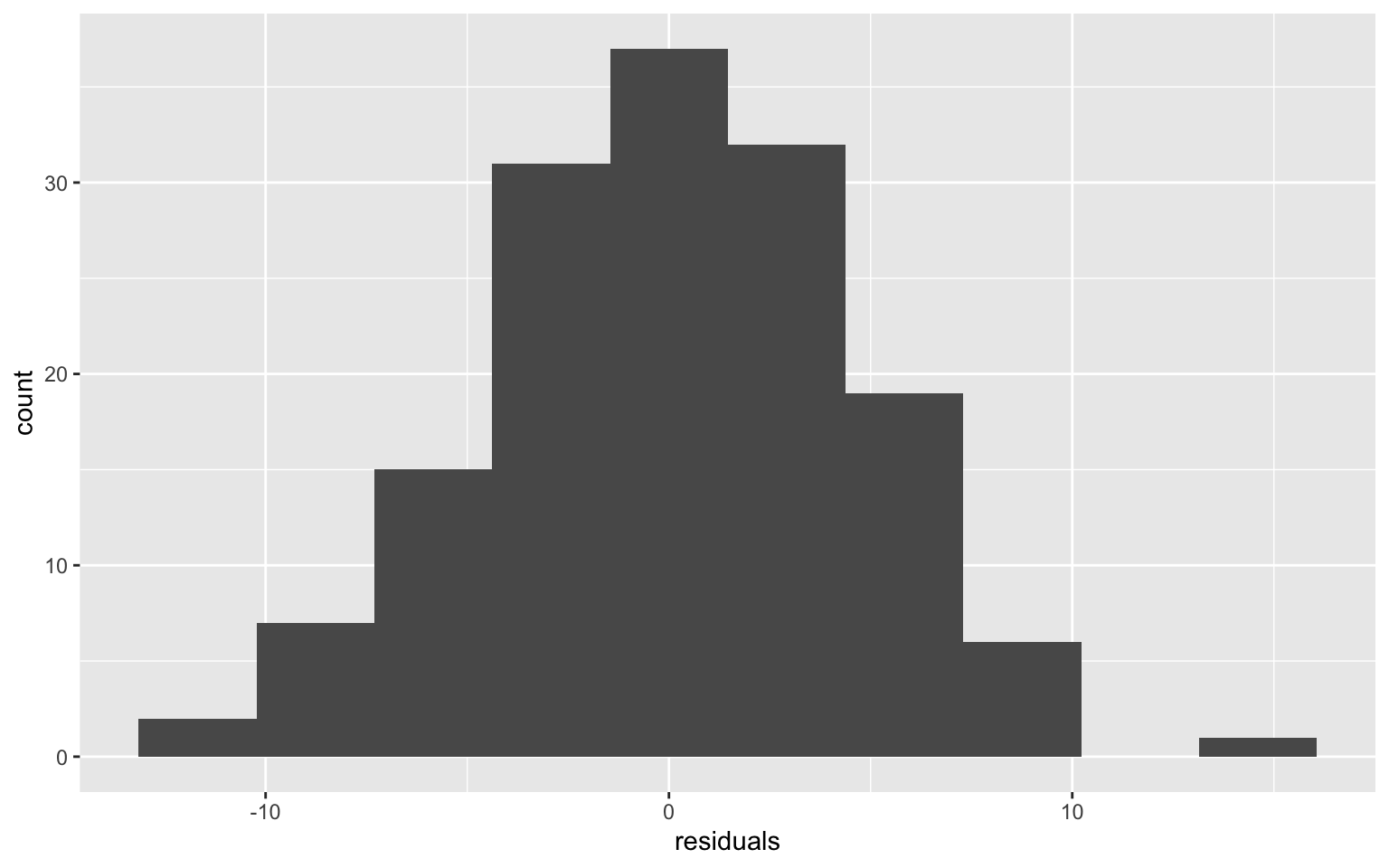
##This plot looks very normal. This assumption has been met.
##double checking with Shapiro-Wilk test
shapiro.test(residuals)
##
## Shapiro-Wilk normality test
##
## data: residuals
## W = 0.99484, p-value = 0.8766##p-value>.05, normal distribution of residuals.
#Homoskedasticity
fitted<-lm(mb ~ timenum*bh_c*bl_c*nh_c, data=skulls2)$fitted.values
ggplot()+geom_point(aes(residuals,fitted))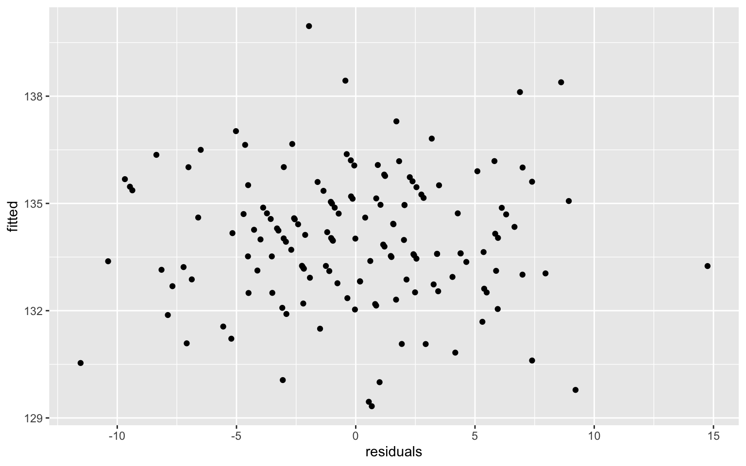
##The scatter is very even. This assumption has been met

#Observations are random and independent of each other.

#All assumptions have been met.
Linear Regression Model
fit1<-lm(mb ~ timenum*bh_c*bl_c*nh_c, data=skulls2)
summary(fit1)
##
## Call:
## lm(formula = mb ~ timenum * bh_c * bl_c * nh_c, data =
skulls2)
##
## Residuals:
## Min 1Q Median 3Q Max
## -11.5366 -2.9941 -0.0245 2.8219 14.7513
##
## Coefficients:
## Estimate Std. Error t value Pr(>|t|)
## (Intercept) 1.336e+02 4.595e-01 290.747 < 2e-16 ***
## timenum 2.657e+00 1.221e+00 2.177 0.03125 *
## bh_c -4.685e-02 9.468e-02 -0.495 0.62155
## bl_c -7.488e-02 8.652e-02 -0.865 0.38835
## nh_c 4.598e-01 1.537e-01 2.991 0.00331 **
## timenum:bh_c 6.328e-02 2.500e-01 0.253 0.80057
## timenum:bl_c -5.253e-02 2.601e-01 -0.202 0.84024
## bh_c:bl_c 9.327e-04 1.986e-02 0.047 0.96260
## timenum:nh_c -4.414e-01 3.507e-01 -1.259 0.21032
## bh_c:nh_c -1.688e-02 2.893e-02 -0.583 0.56057
## bl_c:nh_c 3.379e-02 3.211e-02 1.052 0.29458
## timenum:bh_c:bl_c -1.707e-02 5.491e-02 -0.311 0.75634
## timenum:bh_c:nh_c -5.284e-02 8.578e-02 -0.616 0.53896
## timenum:bl_c:nh_c 4.661e-02 9.166e-02 0.508 0.61199
## bh_c:bl_c:nh_c -5.065e-03 6.154e-03 -0.823 0.41195
## timenum:bh_c:bl_c:nh_c 4.427e-03 1.734e-02 0.255 0.79890
## ---
## Signif. codes: 0 '***' 0.001 '**' 0.01 '*' 0.05 '.' 0.1
' ' 1
##
## Residual standard error: 4.787 on 134 degrees of freedom
## Multiple R-squared: 0.1383, Adjusted R-squared: 0.04189
## F-statistic: 1.434 on 15 and 134 DF, p-value: 0.1401ggplot(skulls2, aes(x = bh_c, y = mb, color = timechar)) + stat_smooth(method = "lm") +
geom_point() + xlab("Basibregmatic Height (mm)") + ylab("Maximum Breath (mm)") +
ggtitle("Maximum Breaths by Basibregmatic Height and Age") +
theme_classic()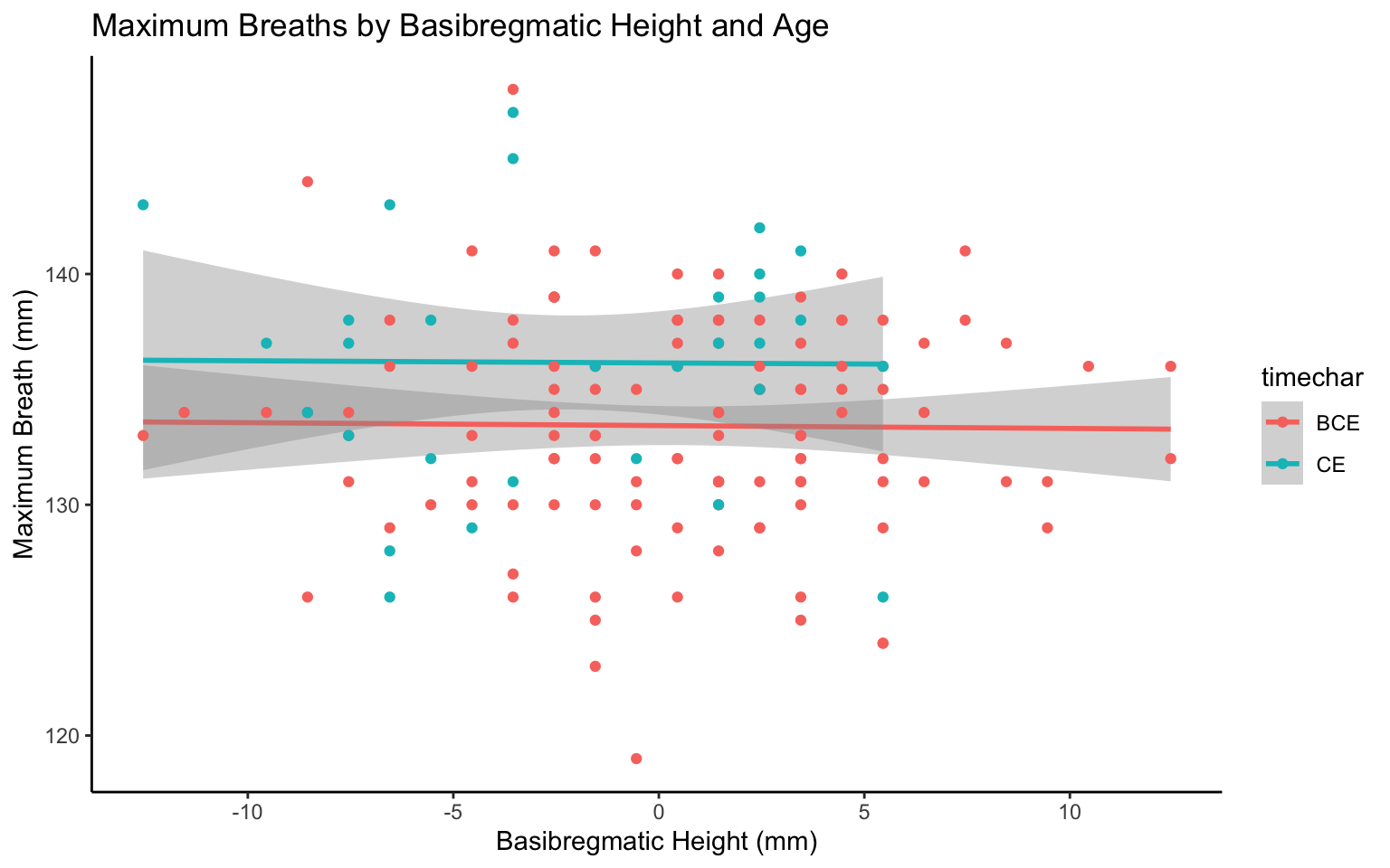 ### Percent of variation predicted by model
4.02% of the variation in maximum breath can be explained by the variation in time, basibregmatic height, basialiveolar length, and nasal height.
### Percent of variation predicted by model
4.02% of the variation in maximum breath can be explained by the variation in time, basibregmatic height, basialiveolar length, and nasal height.
Complete Model and interpretation
mb = .01336 + 2.657(CE) - .04685(bh_c) -.07488(bl_c) + .4598(nh_c) + .06328(CE)(bh_c) - .05253(CE)(bl_c) + .0009327(bh_c)(bl_c) -.4414(CE)(nh_c) -.01688(bh_c)(nh_c) +.03379(bl_c)(nh_c) - .01707(CE)(bh_c)(bl_c) - .05284(CE)(bh_c)(nh_c) + .04661(CE)(bl_c)(nh_c) - .005065(bh_c)(bl_c)(nh_c) +.004427(CE)(bh_c)(bl_c)(nh_c)
This model predicts that for a skull from BCE with an average bh, bl, and nh, their maximum breath would be .01336mm. The coefficient 2.657 predicts that a skull from CE with an average bh, bl, and nh will have a 2.657mm larger maximum breath. The coefficient -.04685 predicts that a skull from BCE with an average bl and nh will have a decrease of -.04685mm in maximum breath for every 1mm increase in bh. The coefficient -.07488 predicts that a skull from BCE with an average bh and nh will have a decrease of -.07488mm in maximum breath for every 1mm increase in bl. The coefficient .4598 predicts that a skull from BCE with an average bh and bl will have a increase of .4598mm in maximum breath for every 1mm increase in nh.
Only of the interactions are significant and are extremely complicated to list and interpret. The interactions between {time & bh}, {bh & bl}, {bl & nh}, {time, bl, & nh}, and {time, bh, bl, & nh} are all positive and indicate that an increase in one of the variables involved results in an increase in all of the variables involved. The rest of the interactions are negative and result in a decrease in all variables involved when there is an increase in one of the variables involved.
Model with Robust Standard Errors
library(sandwich)
library(lmtest)

#Is the model homoskedastic?
bptest(fit1)
##
## studentized Breusch-Pagan test
##
## data: fit1
## BP = 10.965, df = 15, p-value = 0.7551##It is, but the model will have robust standard errors anyway
#Original Coefficients and SEs
summary(fit1)$coef[,1:2]## Estimate Std. Error
## (Intercept) 1.336114e+02 0.459544669
## timenum 2.657204e+00 1.220688955
## bh_c -4.685020e-02 0.094684056
## bl_c -7.487567e-02 0.086519115
## nh_c 4.597593e-01 0.153723913
## timenum:bh_c 6.327553e-02 0.249987863
## timenum:bl_c -5.253262e-02 0.260084828
## bh_c:bl_c 9.327479e-04 0.019855502
## timenum:nh_c -4.414090e-01 0.350683612
## bh_c:nh_c -1.688072e-02 0.028932502
## bl_c:nh_c 3.378750e-02 0.032110154
## timenum:bh_c:bl_c -1.707206e-02 0.054907524
## timenum:bh_c:nh_c -5.283963e-02 0.085782737
## timenum:bl_c:nh_c 4.660515e-02 0.091664864
## bh_c:bl_c:nh_c -5.065239e-03 0.006154283
## timenum:bh_c:bl_c:nh_c 4.427121e-03 0.017342670#Coefficients with robust SEs
coeftest(fit1, vcov = vcovHC(fit1))[,1:2]## Estimate Std. Error
## (Intercept) 1.336114e+02 0.443965686
## timenum 2.657204e+00 2.225740985
## bh_c -4.685020e-02 0.088184976
## bl_c -7.487567e-02 0.096326779
## nh_c 4.597593e-01 0.162060037
## timenum:bh_c 6.327553e-02 0.486532215
## timenum:bl_c -5.253262e-02 0.608059028
## bh_c:bl_c 9.327479e-04 0.023582797
## timenum:nh_c -4.414090e-01 0.599683567
## bh_c:nh_c -1.688072e-02 0.024375676
## bl_c:nh_c 3.378750e-02 0.030006317
## timenum:bh_c:bl_c -1.707206e-02 0.117876355
## timenum:bh_c:nh_c -5.283963e-02 0.155531420
## timenum:bl_c:nh_c 4.660515e-02 0.200991872
## bh_c:bl_c:nh_c -5.065239e-03 0.005182723
## timenum:bh_c:bl_c:nh_c 4.427121e-03 0.037766269#New fit
coeftest(fit1, vcov = vcovHC(fit1))##
## t test of coefficients:
##
## Estimate Std. Error t value Pr(>|t|)
## (Intercept) 1.3361e+02 4.4397e-01 300.9498 < 2.2e-16 ***
## timenum 2.6572e+00 2.2257e+00 1.1939 0.234645
## bh_c -4.6850e-02 8.8185e-02 -0.5313 0.596110
## bl_c -7.4876e-02 9.6327e-02 -0.7773 0.438347
## nh_c 4.5976e-01 1.6206e-01 2.8370 0.005262 **
## timenum:bh_c 6.3276e-02 4.8653e-01 0.1301 0.896719
## timenum:bl_c -5.2533e-02 6.0806e-01 -0.0864 0.931282
## bh_c:bl_c 9.3275e-04 2.3583e-02 0.0396 0.968509
## timenum:nh_c -4.4141e-01 5.9968e-01 -0.7361 0.462975
## bh_c:nh_c -1.6881e-02 2.4376e-02 -0.6925 0.489807
## bl_c:nh_c 3.3787e-02 3.0006e-02 1.1260 0.262173
## timenum:bh_c:bl_c -1.7072e-02 1.1788e-01 -0.1448
0.885062
## timenum:bh_c:nh_c -5.2840e-02 1.5553e-01 -0.3397
0.734587
## timenum:bl_c:nh_c 4.6605e-02 2.0099e-01 0.2319 0.816988
## bh_c:bl_c:nh_c -5.0652e-03 5.1827e-03 -0.9773 0.330166
## timenum:bh_c:bl_c:nh_c 4.4271e-03 3.7766e-02 0.1172
0.906858
## ---
## Signif. codes: 0 '***' 0.001 '**' 0.01 '*' 0.05 '.' 0.1
' ' 1Significance
The significance of the results of this linear model have changed after substituting the SEs for more robust ones. After using robust standard errors, the time variable is no longer significant (original p-value was 0.03125 and the new p-value is 0.234645). The only remaining significant factor in the new model is the variable nasal height (mm) that has been mean centered, none of the interactions were significant. In the original model, the p-value for nh was 0.00331 and the new p-value is 0.005262 which is still significant. From this model, we would be able to reject the null that while controlling for time (BCE or CE), basibregmatic height, and basialiveolar length, nasal height, does not explain variation in maximum breath of Egyptian skulls.
Linear Regression Model with Bootstrapped Standard Errors
samp_skull <- replicate (5000, {
boot_dat <- sample_frac(skulls2, replace=T)
fit2 <- lm(mb ~ timenum*bh_c*bl_c*nh_c, data=boot_dat)
coef(fit2)
})
Comparisons
#Original Coefficients and SEs
summary(fit1)$coef[,1:2]
## Estimate Std. Error
## (Intercept) 1.336114e+02 0.459544669
## timenum 2.657204e+00 1.220688955
## bh_c -4.685020e-02 0.094684056
## bl_c -7.487567e-02 0.086519115
## nh_c 4.597593e-01 0.153723913
## timenum:bh_c 6.327553e-02 0.249987863
## timenum:bl_c -5.253262e-02 0.260084828
## bh_c:bl_c 9.327479e-04 0.019855502
## timenum:nh_c -4.414090e-01 0.350683612
## bh_c:nh_c -1.688072e-02 0.028932502
## bl_c:nh_c 3.378750e-02 0.032110154
## timenum:bh_c:bl_c -1.707206e-02 0.054907524
## timenum:bh_c:nh_c -5.283963e-02 0.085782737
## timenum:bl_c:nh_c 4.660515e-02 0.091664864
## bh_c:bl_c:nh_c -5.065239e-03 0.006154283
## timenum:bh_c:bl_c:nh_c 4.427121e-03 0.017342670#Coefficients with robust SEs
coeftest(fit1, vcov = vcovHC(fit1))[,1:2]## Estimate Std. Error
## (Intercept) 1.336114e+02 0.443965686
## timenum 2.657204e+00 2.225740985
## bh_c -4.685020e-02 0.088184976
## bl_c -7.487567e-02 0.096326779
## nh_c 4.597593e-01 0.162060037
## timenum:bh_c 6.327553e-02 0.486532215
## timenum:bl_c -5.253262e-02 0.608059028
## bh_c:bl_c 9.327479e-04 0.023582797
## timenum:nh_c -4.414090e-01 0.599683567
## bh_c:nh_c -1.688072e-02 0.024375676
## bl_c:nh_c 3.378750e-02 0.030006317
## timenum:bh_c:bl_c -1.707206e-02 0.117876355
## timenum:bh_c:nh_c -5.283963e-02 0.155531420
## timenum:bl_c:nh_c 4.660515e-02 0.200991872
## bh_c:bl_c:nh_c -5.065239e-03 0.005182723
## timenum:bh_c:bl_c:nh_c 4.427121e-03 0.037766269#Coefficients with Bootstrapped SEs
samp_skull %>% t %>% as.data.frame %>% summarize_all(sd)## (Intercept) timenum bh_c bl_c nh_c timenum:bh_c
timenum:bl_c bh_c:bl_c
## 1 0.4299282 1.769838 0.08691601 0.09237108 0.1619333
0.4369331 0.516272 0.02303842
## timenum:nh_c bh_c:nh_c bl_c:nh_c timenum:bh_c:bl_c
timenum:bh_c:nh_c timenum:bl_c:nh_c
## 1 0.5864701 0.02516814 0.0315296 0.1034046 0.1708943
0.1872418
## bh_c:bl_c:nh_c timenum:bh_c:bl_c:nh_c
## 1 0.005667245 0.0375275The SEs from the robust model are larger than that of the original model and the SEs that have been bootstrapped are larger than the robust SEs. Since the standard errors are larger for the bootstrapped SE model, the p-value will be larger, and it will be more difficult to reject the null hypotheses from the original regression.
Logistic Regression
This model will use a logistic regression to predict age (BCE or CE) from the mean-centered measurements of maximum breath (mm), basibregmatic height (mm), basialiveolar length (mm), and nasal height (mm).
###Hypotheses: - The hypotheses are the same as the ones for the linear regression
Assumptions
- The observations are random and independent of each other. True
- The independent variables are each linearly related to the log-odds. True
- There are at lease 10 cases for each outcome. True
Logistic Model
skulls2$timechar <- factor(skulls2$timechar)

logfit <- glm(timechar~mb_c+bh_c+bl_c+nh_c,data=skulls2,family=binomial(link="logit"))
summary(logfit)
##
## Call:
## glm(formula = timechar ~ mb_c + bh_c + bl_c + nh_c,
family = binomial(link = "logit"),
## data = skulls2)
##
## Deviance Residuals:
## Min 1Q Median 3Q Max
## -1.6986 -0.6567 -0.4803 -0.2758 2.6067
##
## Coefficients:
## Estimate Std. Error z value Pr(>|z|)
## (Intercept) -1.65691 0.24970 -6.636 3.23e-11 ***
## mb_c 0.10207 0.04847 2.106 0.0352 *
## bh_c -0.08247 0.04641 -1.777 0.0756 .
## bl_c -0.11010 0.04667 -2.359 0.0183 *
## nh_c 0.05345 0.06836 0.782 0.4343
## ---
## Signif. codes: 0 '***' 0.001 '**' 0.01 '*' 0.05 '.' 0.1
' ' 1
##
## (Dispersion parameter for binomial family taken to be 1)
##
## Null deviance: 150.12 on 149 degrees of freedom
## Residual deviance: 128.89 on 145 degrees of freedom
## AIC: 138.89
##
## Number of Fisher Scoring iterations: 5coeftest(logfit)##
## z test of coefficients:
##
## Estimate Std. Error z value Pr(>|z|)
## (Intercept) -1.656908 0.249696 -6.6357 3.23e-11 ***
## mb_c 0.102072 0.048465 2.1061 0.03520 *
## bh_c -0.082466 0.046408 -1.7770 0.07557 .
## bl_c -0.110098 0.046665 -2.3593 0.01831 *
## nh_c 0.053448 0.068363 0.7818 0.43431
## ---
## Signif. codes: 0 '***' 0.001 '**' 0.01 '*' 0.05 '.' 0.1
' ' 1exp(coef(logfit))## (Intercept) mb_c bh_c bl_c nh_c
## 0.1907279 1.1074633 0.9208426 0.8957465 1.0549026Interpretation of Coefficients
- The odds of age (BCE or CE) for skulls with an average mb, bh, bl, and nh is 0.1907.
- Controlling for bh, bl, and nh, for every 1 mm increase in maximum breath, the odds of age being CE increase by a factor of 1.1075 (This is significant with p-value=0.0352).
- Controlling for mb, bl, and nh, for every 1 mm increase in basibregmatic height, the odds of age being CE increase by a factor of 0.9208 (This is not significant with p-value=0.0756).
- Controlling for mb, bh, and nh, for every 1 mm increase in basialiveolar length, the odds of age being CE increase by a factor of 0.8957 (This is significant with p-value=0.0183).
- Controlling for mb, bh, and bl, for every 1 mm increase in nasal height, the odds of age being CE increase by a factor of 1.0549 (This is not significant with p-value=0.4343).
Confisuion Matrix
probs<-predict(logfit,type="response")
table(predict=as.numeric(probs>.5),truth=skulls2$timechar)%>%addmargins
## truth
## predict BCE CE Sum
## 0 117 24 141
## 1 3 6 9
## Sum 120 30 150#Sensitivity (TPR)
6/30## [1] 0.2#The true positive rate or sensitivity for this model is 20%.
#Which means that the model accuratly predicts CE 20% of the time
#Specificity (TNR)
117/120## [1] 0.975#The true negative rate or sensitivity for this model is 97.5%.
#Which means that the model accuratly predicts BCE 97.5% of the time
#Precision
6/9## [1] 0.6666667#The positive rate or precision for this model is 66.66%.
#Which means that the model CE 66.66% of the time.
#Accuracy
(117+6)/150## [1] 0.82#The accuracy rate of this model is 82%.
#Which means that it is accurate 82% of the time.Density Plot of log-odds by Age (timchar) variable
skulls2$logit<-predict(logfit,type="link")

skulls2%>%ggplot()+
  geom_density(aes(logit,color=timechar,fill=timechar), alpha=.4)+
  theme(legend.position=c(.85,.85)) +
  geom_vline(xintercept=0)+
  xlab("predictor (logit)")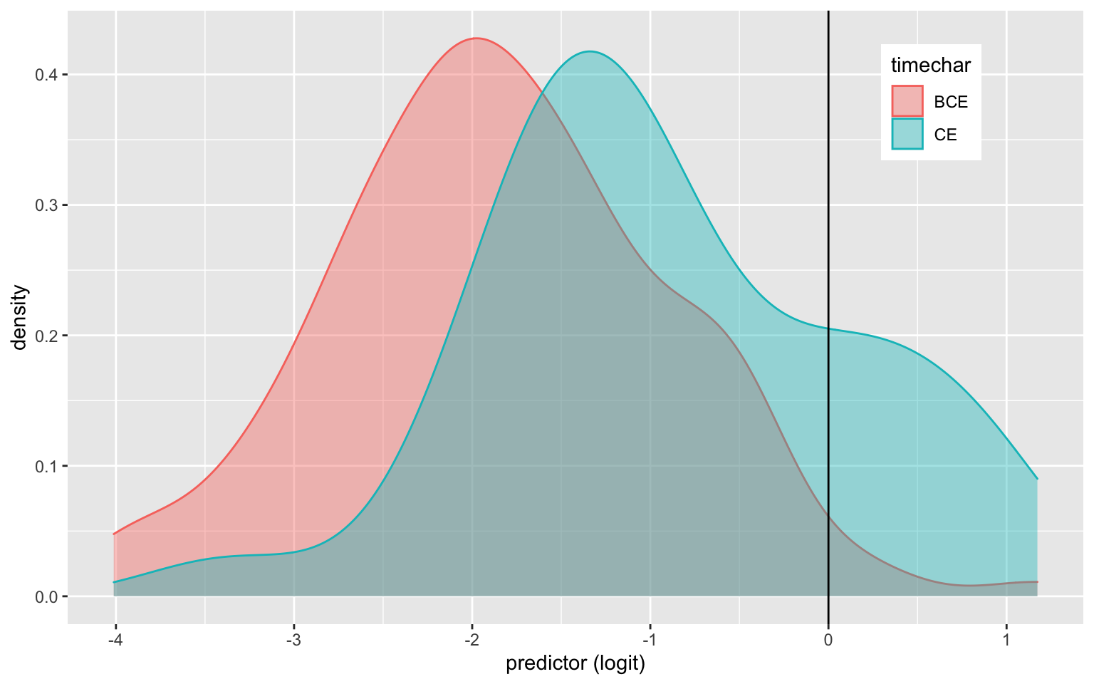
ROC Curve
#Creating prob and truth variables in new dataset
skulls2<-skulls2%>%mutate(prob=predict(logfit, type="response"), predict=ifelse(prob>.5,1,0))
class<-skulls2%>%transmute(prob,predict,truth=skulls2$timechar)
class
## prob predict truth
## 1 0.15549700 0 BCE
## 2 0.10802907 0 BCE
## 3 0.09579425 0 BCE
## 4 0.03046857 0 BCE
## 5 0.07324186 0 BCE
## 6 0.37261576 0 BCE
## 7 0.08618579 0 BCE
## 8 0.06701567 0 BCE
## 9 0.06376682 0 BCE
## 10 0.11404008 0 BCE
## 11 0.07561986 0 BCE
## 12 0.39394169 0 BCE
## 13 0.02777784 0 BCE
## 14 0.07025724 0 BCE
## 15 0.12559165 0 BCE
## 16 0.12176758 0 BCE
## 17 0.06360842 0 BCE
## 18 0.19713210 0 BCE
## 19 0.19343412 0 BCE
## 20 0.08834919 0 BCE
## 21 0.04251203 0 BCE
## 22 0.06388218 0 BCE
## 23 0.38746602 0 BCE
## 24 0.04084007 0 BCE
## 25 0.05808916 0 BCE
## 26 0.16512168 0 BCE
## 27 0.15056987 0 BCE
## 28 0.03614766 0 BCE
## 29 0.01776864 0 BCE
## 30 0.02007215 0 BCE
## 31 0.02228621 0 BCE
## 32 0.10984320 0 BCE
## 33 0.13558827 0 BCE
## 34 0.31880476 0 BCE
## 35 0.12760122 0 BCE
## 36 0.12461490 0 BCE
## 37 0.04264981 0 BCE
## 38 0.09005464 0 BCE
## 39 0.11110601 0 BCE
## 40 0.24476106 0 BCE
## 41 0.06595078 0 BCE
## 42 0.06546269 0 BCE
## 43 0.09500257 0 BCE
## 44 0.16265124 0 BCE
## 45 0.04449196 0 BCE
## 46 0.11183488 0 BCE
## 47 0.11884769 0 BCE
## 48 0.04126056 0 BCE
## 49 0.05115137 0 BCE
## 50 0.28918926 0 BCE
## 51 0.05806248 0 BCE
## 52 0.05266291 0 BCE
## 53 0.13712961 0 BCE
## 54 0.25475341 0 BCE
## 55 0.05789175 0 BCE
## 56 0.22122170 0 BCE
## 57 0.07389525 0 BCE
## 58 0.17087443 0 BCE
## 59 0.18054284 0 BCE
## 60 0.10121392 0 BCE
## 61 0.12593083 0 BCE
## 62 0.11596345 0 BCE
## 63 0.19414436 0 BCE
## 64 0.03617494 0 BCE
## 65 0.11501387 0 BCE
## 66 0.21440519 0 BCE
## 67 0.14866621 0 BCE
## 68 0.07314783 0 BCE
## 69 0.25065222 0 BCE
## 70 0.08915490 0 BCE
## 71 0.20837057 0 BCE
## 72 0.12031092 0 BCE
## 73 0.18848382 0 BCE
## 74 0.31486844 0 BCE
## 75 0.01826213 0 BCE
## 76 0.08359966 0 BCE
## 77 0.12722590 0 BCE
## 78 0.54090595 1 BCE
## 79 0.21222928 0 BCE
## 80 0.21907624 0 BCE
## 81 0.27087841 0 BCE
## 82 0.11221214 0 BCE
## 83 0.20771688 0 BCE
## 84 0.09958557 0 BCE
## 85 0.27098597 0 BCE
## 86 0.34318018 0 BCE
## 87 0.10403013 0 BCE
## 88 0.15691032 0 BCE
## 89 0.18913033 0 BCE
## 90 0.27972480 0 BCE
## 91 0.07839603 0 BCE
## 92 0.42713948 0 BCE
## 93 0.55194303 1 BCE
## 94 0.15438025 0 BCE
## 95 0.40513180 0 BCE
## 96 0.18222089 0 BCE
## 97 0.34218724 0 BCE
## 98 0.40628086 0 BCE
## 99 0.39011976 0 BCE
## 100 0.10035560 0 BCE
## 101 0.25463883 0 BCE
## 102 0.15848009 0 BCE
## 103 0.11066520 0 BCE
## 104 0.13903998 0 BCE
## 105 0.21377501 0 BCE
## 106 0.17030248 0 BCE
## 107 0.06181463 0 BCE
## 108 0.08193430 0 BCE
## 109 0.37045900 0 BCE
## 110 0.36275831 0 BCE
## 111 0.36528216 0 BCE
## 112 0.76370204 1 BCE
## 113 0.31840190 0 BCE
## 114 0.11983253 0 BCE
## 115 0.29178877 0 BCE
## 116 0.35398623 0 BCE
## 117 0.07807605 0 BCE
## 118 0.19598823 0 BCE
## 119 0.16867243 0 BCE
## 120 0.15080737 0 BCE
## 121 0.49763914 0 CE
## 122 0.22009982 0 CE
## 123 0.30973642 0 CE
## 124 0.16324527 0 CE
## 125 0.53815255 1 CE
## 126 0.03346198 0 CE
## 127 0.17058212 0 CE
## 128 0.14716952 0 CE
## 129 0.13290203 0 CE
## 130 0.33376678 0 CE
## 131 0.61383112 1 CE
## 132 0.17358935 0 CE
## 133 0.21033916 0 CE
## 134 0.27360238 0 CE
## 135 0.28246460 0 CE
## 136 0.21195790 0 CE
## 137 0.28912497 0 CE
## 138 0.20821268 0 CE
## 139 0.33341889 0 CE
## 140 0.59198723 1 CE
## 141 0.21360622 0 CE
## 142 0.10929613 0 CE
## 143 0.71088333 1 CE
## 144 0.46732571 0 CE
## 145 0.19728368 0 CE
## 146 0.70273382 1 CE
## 147 0.49238146 0 CE
## 148 0.10708277 0 CE
## 149 0.70056188 1 CE
## 150 0.17605378 0 CE#Confusion matrix
table(predict=class$predict,truth=class$truth)%>%addmargins()## truth
## predict BCE CE Sum
## 0 117 24 141
## 1 3 6 9
## Sum 120 30 150library(plotROC)
ROC1<-ggplot(class)+geom_roc(aes(d=class$truth,m=class$prob), n.cuts=0)
ROC1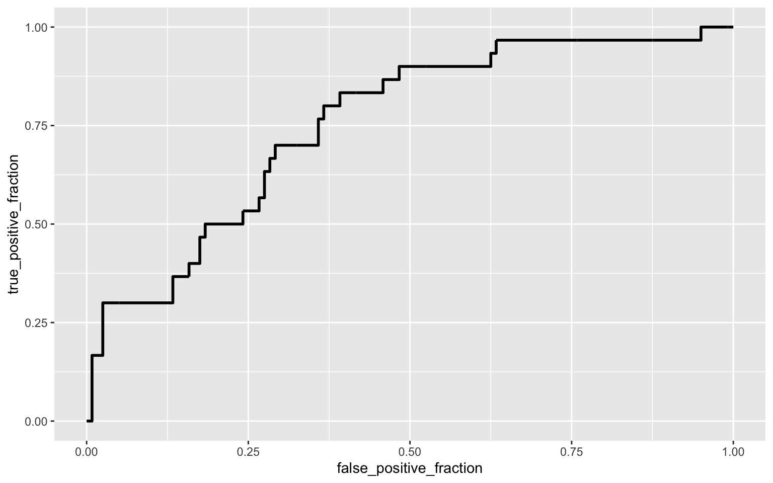
calc_auc(ROC1)## PANEL group AUC
## 1 1 -1 0.7547222This ROC curve has a fair AUC of .7547222 which suggests that 75.47% of the data is explained by the model. The ROC curve helps show the AUC and how much of the data, that the model does not explain (area above the curve).
10-fold CV
class_diag<-function(probs,truth){
  if(is.numeric(truth)==FALSE & is.logical(truth)==FALSE) truth<-as.numeric(truth)-1
  tab<-table(factor(probs>.5,levels=c("FALSE","TRUE")),truth)
  prediction<-ifelse(probs>.5,1,0)
  acc=mean(truth==prediction)
  sens=mean(prediction[truth==1]==1)
  spec=mean(prediction[truth==0]==0)
  ppv=mean(truth[prediction==1]==1)
  ord<-order(probs, decreasing=TRUE)
  probs <- probs[ord]; truth <- truth[ord]
  TPR=cumsum(truth)/max(1,sum(truth))
  FPR=cumsum(!truth)/max(1,sum(!truth))
  dup<-c(probs[-1]>=probs[-length(probs)], FALSE)
  TPR<-c(0,TPR[!dup],1); FPR<-c(0,FPR[!dup],1)
  n <- length(TPR)
  auc<- sum( ((TPR[-1]+TPR[-n])/2) * (FPR[-1]-FPR[-n]) )
  data.frame(acc,sens,spec,ppv,auc)
}

set.seed(1234)
k=10

data<-skulls2[sample(nrow(skulls2)),]
folds<-cut(seq(1:nrow(skulls2)),breaks=k,labels=F)
diags<-NULL
for(i in 1:k){
  train<-data[folds!=i,]
  test<-data[folds==i,]
  truth<-test$timechar
  fit<-glm(timechar~mb_c+bh_c+bl_c+nh_c,data=train,family="binomial")
  probs<-predict(fit,newdata = test,type="response")
  diags<-rbind(diags,class_diag(probs,truth))
}
summarize_all(diags,mean)
## acc sens spec ppv auc
## 1 0.8133333 0.125 0.9711966 NaN 0.7103114The logistic regression performed decently well with the sample data and had a fair AUC of 0.7547222. This is a start difference from the 10-fold CV using the model which had a poor AUC of 0.656864. This suggests that the model is overfitted to the original sample and is less useful for different samples/real world populations. This could be helped using the lasso regression method.
Lasso Regression 10-CV
Lasso
library(glmnet)
y <- as.matrix(skulls2$timechar)
x <- model.matrix(timechar~mb_c+bh_c+bl_c+nh_c, data=skulls2)
cv<-cv.glmnet(x,y,family='binomial')
lasso1<-glmnet(x,y, family="binomial",lambda=cv$lambda.1se)
coef(lasso1)
## 6 x 1 sparse Matrix of class "dgCMatrix"
## s0
## (Intercept) -1.386294
## (Intercept) 0.000000
## mb_c .
## bh_c .
## bl_c .
## nh_c .lasso2<-glmnet(x,y, family="binomial",lambda=cv$lambda.min)
coef(lasso2)## 6 x 1 sparse Matrix of class "dgCMatrix"
## s0
## (Intercept) -1.59003062
## (Intercept) .
## mb_c 0.08671316
## bh_c -0.06934533
## bl_c -0.09703462
## nh_c 0.02914163A lasso regression was calculated to show which variables (mb, bh, bl, and nh) are significant in predicting the age of a skull (BCE or CE). This is what was used for the logistic regression model so the fit of the model can be compared as the logistic model from the previous section had overfitting. Originally, lambda.1se was used in the lasso, but this led to none of the variables being predictor variables. After that, lamba.min was used and now maximum breath, basibregmatic height, and basialiveolar length are the only variables viable for this model.
10-fold using lasso model
set.seed(1234)
k=10

data1<-skulls2[sample(nrow(skulls2)),]
folds<-cut(seq(1:nrow(skulls2)),breaks=k,labels=F)
diags2<-NULL
for(i in 1:k){
  train<-data1[folds!=i,]
  test<-data1[folds==i,]
  truth<-test$timechar
  fit3<-glm(timechar~mb_c+bh_c+bl_c,data=train,family="binomial")
  probs<-predict(fit3,newdata = test,type="response")
  diags2<-rbind(diags,class_diag(probs,truth))
}

diags2%>%summarize_all(mean)
## acc sens spec ppv auc
## 1 0.8181818 0.1136364 0.9738151 NaN 0.6702132When comparing this 10-fold lasso model to the original logistic model and the 10-fold CV for it, it is quite shocking that the AUC has decreased with the more limited model scope. This could be due to the initial lasso (lambda.1se). The first lasso showed that none of the predictor variables were suitable to predict age (timechar), so an additional lasso (lambda.min) was used. Though the original model was overfitted to the training sample, it has a better fit, than this lasso model and does a better of predicting age (BCE or CE) of Egyptian skulls using all 4 variables than the lasso model does with only maximum breath, basibregmatic height, and basialiveolar length.